Chapter 18: Using the Eddy Dissipation and Steady Diffusion Flamelet Combustion Models

This tutorial is divided into the following sections:

18.1. Introduction

This tutorial examines the reacting flow through a can combustor that burns methane in air in order to determine the combustor performance. In this tutorial, you will first mesh the geometry in the Ansys Fluent Meshing and then simulate the combustion process using the Eddy Dissipation model. You will then repeat the simulation using the steady flamelet model and compare the results of these two approaches.

This tutorial demonstrates how to do the following:

Mesh the geometry in Ansys Fluent Meshing.
Set up a combustion simulation in Ansys Fluent.
Set up a reacting flow involving fuel and oxidizer.
Use the Eddy Dissipation model.
Use the Steady Diffusion Flamelet model.
Display the results obtained using these two models.

18.2. Prerequisites

This tutorial is written with the assumption that you have completed the introductory tutorials found in this manual and that you are familiar with the Ansys Fluent outline view and ribbon structure. Some steps in the setup and solution procedure will not be shown explicitly.

18.3. Problem Description

A can type combustor is a component of a land-based gas turbine in which combustion occurs. Can combustors are designed to burn the fuel efficiently, minimize the emissions, and reduce the wall temperature. The can combustor to be considered in this tutorial is shown schematically in Figure 18.1: Can Combustor Geometry.

Figure 18.1: Can Combustor Geometry

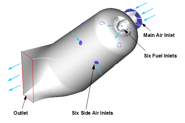
Compressed primary air is forced into the combustion chamber at 10 m/s through the main inlet at the base of the canister. Six swirl inlet vanes guide the incoming air into the canister and facilitate its mixing with pure methane for proper combustion. Methane is injected through six fuel inlets with a velocity of 40 m/s. As the reacting mixture proceeds through the canister, secondary air is fed into the combustion chamber at a velocity of 6 m/s through six secondary air inlets downstream from the primary combustion zone. This helps increase the combustion efficiency and also cool the can walls as they are exposed to the hot reacting flow. The fuel and oxidizer enter the combustion chamber at 300 K.

In this tutorial, the quantitative analysis of the combusting mixture is performed and the following quantities are determined:

The expected loss of total pressure through the combustor
The temperature distribution inside the combustor that burns methane in air
The proportion of unburned fuel remaining at the combustor outlet

18.4. Setup and Solution

The following sections describe the setup and solution steps for this tutorial:

You can also watch a video that demonstrates how to setup, solve, and postprocess the solution results for diffusion-controlled combustion at:

18.4.1. Preparation

To prepare for running this tutorial:

Download the edm_flamelet.zip file here .
Unzip edm_flamelet.zip to your working directory.
The file can_combustor.pmdb can be found in the folder.
Use the Fluent Launcher to start Ansys Fluent.
Select Meshing in the top-left selection list to start Fluent in Meshing Mode.
Enable Double Precision under Options.
Set Meshing Processes and Solver Processes to 4 under Parallel (Local Machine).

18.4.2. Meshing Workflow

In the Workflow tab on the left of the interface, click the drop-down list and select Watertight Geometry.
Import the CAD geometry (can_combustor.pmdb).
1. Select the Import Geometry task.
2. Enable Advanced Options to expose additional options that may be required when importing a CAD geometry.
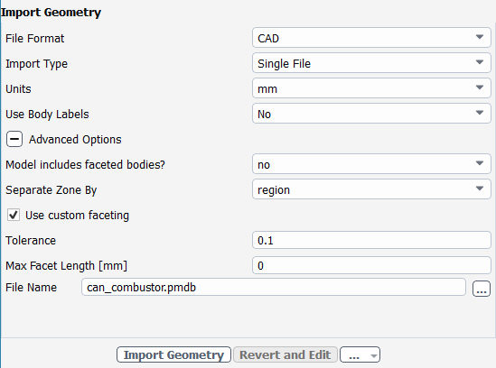
3. Select region for the Separate Zone By.
4. Enable the checkbox beside Use custom faceting.
5. Enter 0.1 for the Tolerance.
6. Locate the can_combustor.pmdb file using the File Name option and select the file.
7. Select Import Geometry.
Add local sizing.
1. Select yes to add local face sizing to the inlets.
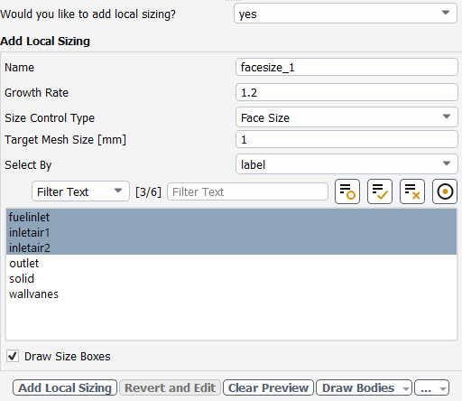
  1. Select Face Size for the Size Control Type.
  2. Change the Target Mesh Size to 1.
  3. Select fuelinlet, inletair1 and inletair2 from the list of labels.
  4. Click Add Local Sizing.
2. Add fuelinlet proximity sizing.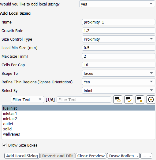
  1. Change the Size Control Type to Proximity.
  2. Adjust the Local Min Size to be 0.5 and the Max Size to be 2.
  3. Change the number of Cells Per Gap to be 16.
  4. Select fuelinlet from the list of labels and click Add Local Sizing.
3. Add proximity sizing to the inlet vanes.
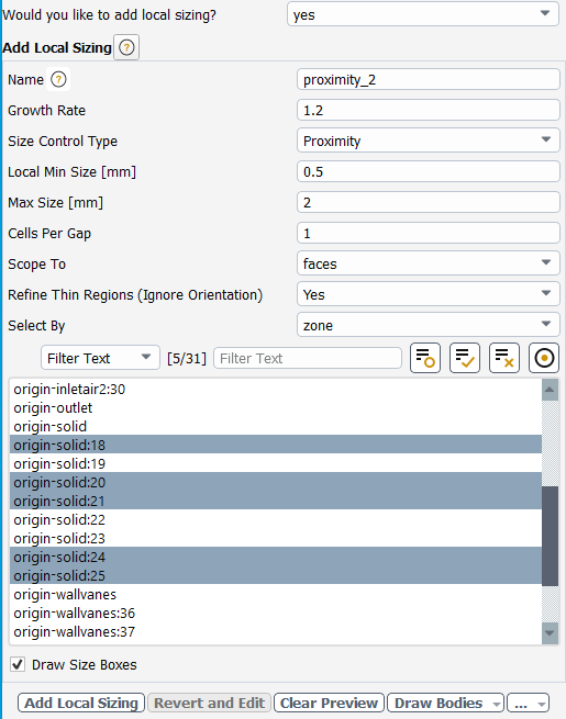
  1. Ensure Proximity is selected and change the Local Min Size to 0.5 and the Max Size to 2.
  2. Change the Select By option to zone.
  3. Select origin-solid:18, origin-solid:20, origin-solid:21, origin-solid:24 and origin-solid:25 from the list of zones.
  4. Click Add Local Sizing.
4. Add face sizing to the inlet vanes.
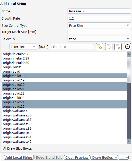
  1. Change the Size Control Type to Face Size and enter 1 for the Target Mesh Size.
  2. Select origin-solid:18, origin-solid:20, origin-solid:21, origin-solid:24 and origin-solid:25 from the list of zones.
  3. Click Add Local Sizing.
Generate the surface mesh.
1. Adjust the Minimum Size to be 1 and the Maximum Size to be 15.
2. Change the Cells Per Gap to be 4 and click 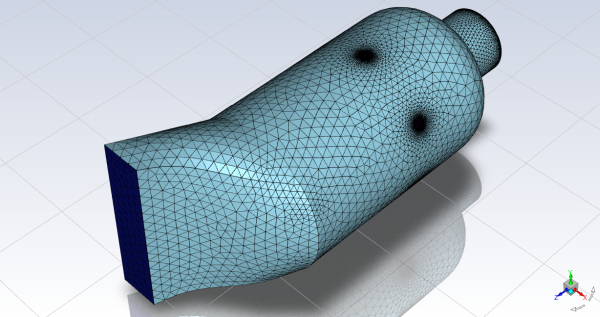Generate the Surface Mesh.
Describe the geometry.
1. In the Describe Geometry task, select the option "The geometry consists of only fluid regions with no voids".
2. Check that both remaining options are set to "No".
3. Click Describe Geometry.
Update the boundaries.
1. Change the wallvanes boundary type to wall.
2. Click Update Boundaries.
Update the regions.
1. Retain default settings and click Update Regions.
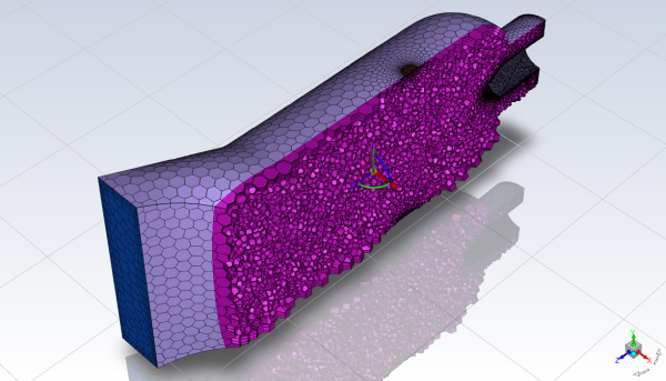
Add boundary layers.
1. Retain default settings and click Add Boundary Layers.
Generate the volume mesh.
1. Change the Max Cell Length to 7.5.
2. Click Generate the Volume Mesh to generate the mesh.
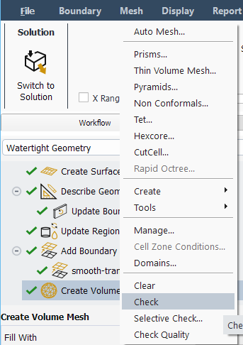
Check the quality of the mesh
1. Select Check from the Mesh drop-down list on the main taskbar.
2. Switch to solution mode by clicking the Switch to Solution button on the Fluent ribbon tab.

18.4.3. Solver Settings

Retain the default setting of Pressure-Based in the Solver group box, under Type. Retain the default selection of Steady from the Time list.
Setup → General

18.4.4. Models

The fuel (methane) and oxidizer (air) undergo fast combustion (that is, the overall combustion rate is controlled by turbulent mixing). In this first part of the tutorial, the combustion reaction is considered to be driven by turbulent diffusion, and it is modeled using the Eddy Dissipation model, which is suitable for modeling fast combustion.

Enable the k-ω SST turbulence model.
Physics → Models → Viscous...
1. Retain the default selections in the Viscous Model dialog box.
2. Click OK to close the Viscous Model dialog box.
Enable chemical species transport and reaction.
Physics → Models → Species...
1. Select Species Transport in the Model list.
2. Select methane-air from the Mixture Material drop-down list.
  The Mixture Material list contains the set of chemical mixtures that exist in the Ansys Fluent database. When selecting an appropriate mixture for your case, you can review the constituent species and the reactions of the predefined mixture by clicking View... next to the Mixture Material drop-down list. The chemical species and their physical and thermodynamic properties are defined by the selection of the mixture material. After enabling the Species Transport model, you can alter the mixture material selection or modify the mixture material properties using the Create/Edit Materials dialog box.
3. Select Volumetric in the Reactions group box.
4. Select Eddy-Dissipation in the Turbulence-Chemistry Interaction group box.
  The Eddy-Dissipation model computes the reaction rate under the assumption that chemical reaction is fast compared to transport of reactants in the combusting flow. That is, the reaction is controlled by diffusion.
5. Click OK to close the Species Model dialog box.
  A Warning message appears in the console notifying you that Ansys Fluent automatically enabled the energy equation required for the Species reaction model.

18.4.5. Boundary Conditions

In this step, you will define the boundary conditions at the inlets and the outlet.

Set the boundary condition for the fuel inlet.

Setup → Boundary Conditions → Inlet → fuelinlet Edit...

In the Velocity Inlet dialog box, configure the following settings.

Tab	Setting	Value
Momentum	Velocity Magnitude	`40` m/s
Thermal	Temperature	`300` (default)
Species	ch4 (Species Mass Fractions group box)	`1`

Set the boundary condition for the primary air inlet.

Setup → Boundary Conditions → Inlet → inletair1 Edit...

In the Velocity Inlet dialog box, configure the following settings.

Tab	Setting	Value
Momentum	Velocity Magnitude	`10` m/s
Thermal	Temperature	`300` (default)
Species	o2 (Species Mass Fractions group box)	`0.23`^[a]
Dry air is composed of 23% of oxygen and 77% of nitrogen, which is a bulk species in the mixture. Ansys Fluent adds an appropriate amount of nitrogen at the boundaries to ensure that the sum of the mass fractions of the components is equal to unity.

Set the boundary condition for the secondary air inlet.

Setup → Boundary Conditions → Inlet → inletair2 Edit...

In the Velocity Inlet dialog box, configure the following settings.

Tab	Setting	Value
Momentum	Velocity Magnitude	`6` m/s
Thermal	Temperature	`300` (default)
Species	o2 (Species Mass Fractions group box)	`0.23`

Set the boundary condition for the pressure outlet.

Setup → Boundary Conditions → Outlet → outlet Edit...

In the Pressure Outlet dialog box, configure the following settings.

Tab	Setting	Value
Momentum	Gauge Pressure	`0` Pa ^[a] (default)
	Backflow Pressure Specification	Total Pressure^[b] (default)
	Average Pressure Specification	(Selected)
The gauge pressure of 0 Pa means that the pressure equals the ambient pressure. This setting ensures that if the backflow occurs, only pure nitrogen at 300 K enters the chamber, which will not affect the combustion reactions.

For wall-part-fluid, wallvanes and wallvanes-shadow retain the default stationary no slip adiabatic settings.

18.4.6. Solution

Specify the discretization schemes.

Solution → Solution → Methods...

In the Solution Methods task page, configure the following settings.

Group Box	Setting	Value
Pressure Velocity Coupling	Scheme	Coupled
N/A	Pseudo Time Method	Global Time Step
N/A	Warped-Face Gradient Correction	(Default) ^[a]
N/A	High Order Term Relaxation	(Enabled)^[b]
The warped-face gradient correction is designed to improve gradient accuracy for all gradient methods. The relaxation of high order terms will help to improve the solution behavior of flow simulations when higher order spatial discretizations are used (higher than first).

Ensure that the plotting of residuals is enabled during the calculation.
Solution → Reports → Residuals...

Create a surface report definition of mass-weighted average of co2 at the outlet.

Solution → Reports → Definitions → New → Surface Report → Mass-Weighted Average...

Configure the following settings.

Group Box	Setting	Value
N/A	Name	`co2-out`
N/A	Field Variable	Species... and Mass fraction of co2
N/A	Surfaces	outlet
Create	Report File	(Selected)
	Report Plot	(Selected)
	Print to Console	(Selected)

Initialize the solution.
Solution → Initialization → Initialize
Save the case file (can_combustor_edm.cas.h5).
File → Write → Case...
Start calculation.
Solution → Run Calculation → Run Calculation...
1. Set the global Time Scale Factor to 5.
  The Time Scale Factor allows you to further manipulate the computed time step size calculated by Ansys Fluent. Larger time steps can lead to faster convergence. However, if the time step is too large it can lead to solution instability.
2. Enter 500 for Number of Iterations.
3. Click Calculate.
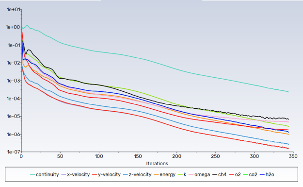
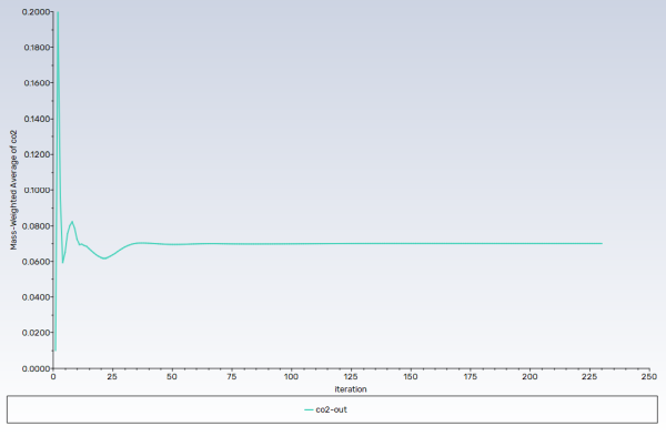
All scaled residuals have met the criteria for a converged solution (Figure 18.2: Scaled Residuals), and the relative amount of CO₂ exiting the combustor outlet has become stable (Figure 18.3: Convergence History of Mass-Weighted Average CO₂ on the Outlet).
Figure 18.2: Scaled Residuals

Figure 18.3: Convergence History of Mass-Weighted Average CO₂ on the Outlet
Save the case and data files (can_combustor_edm.cas.h5 and can_combustor_edm.dat.h5).
File → Write → Case & Data...

18.4.7. Postprocessing for the Eddy-Dissipation Solution

Check the mass flux balance.
Results → Reports → Fluxes...

Warning: Although the mass flow rate history indicates that the solution is converged, you should also check the net mass fluxes through the domain to ensure that mass is being conserved.
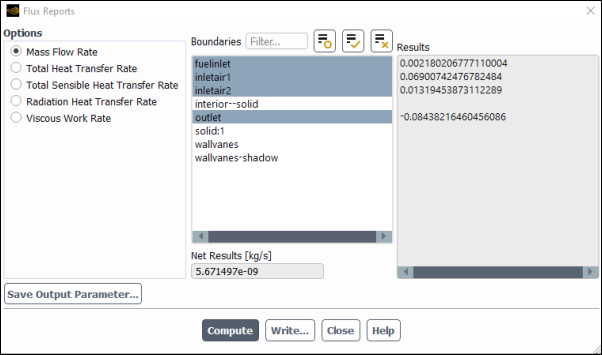
1. Select fuelinlet, inletair1, inletair2 and outlet from the Boundaries selection list.
2. Retain the default Mass Flow Rate option.
3. Click Compute and close the Flux Reports dialog box.
Warning: The net mass imbalance should be a small fraction (for example, 0.5%) of the total flux through the system. If a significant imbalance occurs, you should decrease the residual tolerances by at least an order of magnitude and continue iterating.
Report the total sensible heat flux.
Results → Reports → Fluxes...
1. Select Total Sensible Heat Transfer Rate in the Options list.
2. Select all the boundaries from the Boundaries selection list (you can click the select-all button ( ).
3. Click Compute and close the Flux Reports dialog box.
  Note: The energy balance is good because the net result is small compared to the heat of reaction.
Create an XZ plane, which will be used for plotting the results.
Results → Surface → Create → Plane...
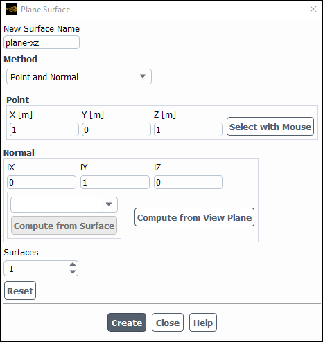
1. Enter plane_xz in for New Surface Name.
2. In the Method drop-down list, select Point and Normal.
3. In the Point group box, enter 1, 0, 1 for X, Y, Z, respectively.
4. In the Normal group box, enter 0, 1, 0 for iX, iY, iZ, respectively.
5. Click Create and close the Plane Surface dialog box.
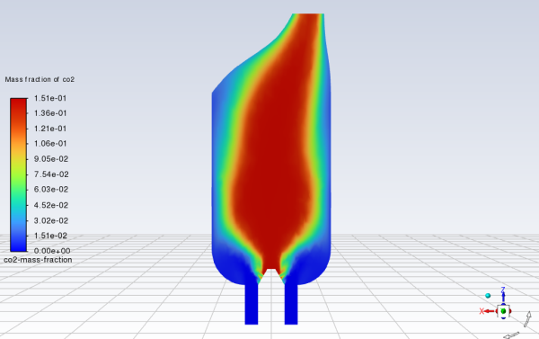
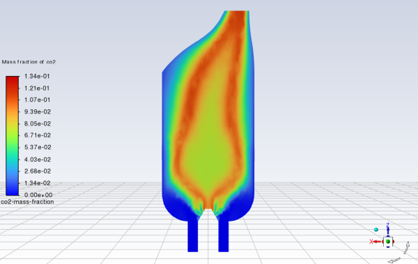
Display filled contours of CO₂ mass fraction in the combustion chamber (Figure 18.4: Contours of CO₂ Mass Fraction).
Results → Graphics → Contours → New...
1. Enter co2-mass-fraction for Contour Name.
2. Enable Filled in the Options group box.
3. From the Contours of drop-down lists, select Species... and Mass Fraction of co2.
4. From the Surfaces selection list, deselect all surfaces and select plane_xz.
5. In the Coloring group box, select Smooth.
6. Click Save/Display, close the Contours dialog box, and rotate the view as shown in Figure 18.4: Contours of CO₂ Mass Fraction.
  Figure 18.4: Contours of CO₂ Mass Fraction
  
  The contour map of the CO₂ concentration shows that the flow is mixing and reacting properly in the combustor.
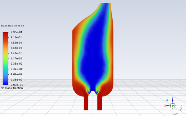
Display filled contours of oxygen mass fraction on the surface plane_xz (Figure 18.5: Contours of O₂ Mass Fraction).
Results → Graphics → Contours → New...
1. Enter o2-mass-fraction for Contour Name.
2. Enable Filled in the Options group box.
3. From the Contours of drop-down lists, select Species... and Mass Fraction of o2.
4. From the Surfaces selection list, deselect all surfaces and select plane_xz.
5. In the Coloring group box, select Smooth.
6. Click Save/Display and close the Contours dialog box.
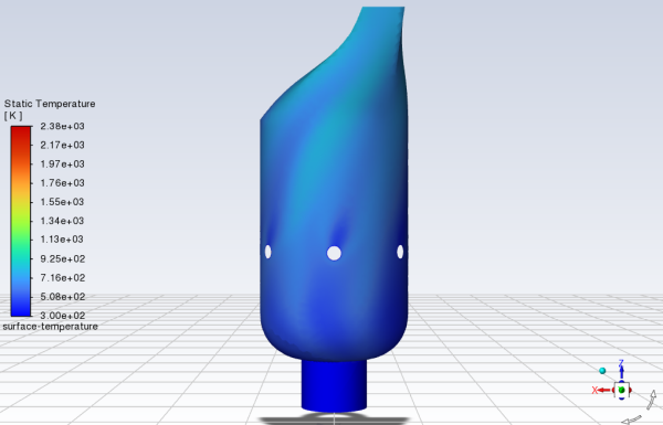
  Figure 18.5: Contours of O₂ Mass Fraction
Display filled contours of temperature on the aluminum combustor walls (Figure 18.6: Contours of Static Temperature on the Combustor Walls).
Results → Graphics → Contours → New...
1. Enter surface-temperature for Contour Name.
2. Enable Filled in the Options group box.
3. From the Contours of drop-down lists, select Temperature... and Static Temperature.
4. Click New Surface and select Iso-Clip.
5. Name the surface clip-y-coordinate and select Mesh... and Y-Coordinate from the Clip to Values of drop-down lists.
6. Select the surface solid:1.
7. Click Compute and enter 0 for the Min (m).
8. Click Create and close the dialog box.
9. From the Surfaces selection list, deselect all surfaces and select clip-y-coordinate and wallvanes.
10. In the Coloring group box, select Smooth.
11. Click Save/Display and close the Contours dialog box.
  Figure 18.6: Contours of Static Temperature on the Combustor Walls
12. Rotate the contour plot to examine the temperature field of the combusting flow on the canister walls from different angles.
Save the case and data files (can_combustor_edm.cas.h5 and can_combustor_edm.dat.h5).
File → Write → Case & Data...

18.5. Steady Diffusion Flamelet Model Setup and Solution

In the first part of the tutorial, the combustion reaction was modeled using the Eddy Dissipation model. In this part of the tutorial, you will use the Steady Diffusion Flamelet model to simulate a turbulent non-premixed reacting flow. The Steady Diffusion Flamelet model can model local chemical non-equilibrium due to turbulent strain.

In the Steady Diffusion Flamelet model, reactions take place in a thin laminar locally one-dimensional zone, called 'flamelet'. The turbulent flame is represented by an ensemble of such flamelets. Detailed chemical kinetics is used to describe the combustion reaction. The chemistry is assumed to respond rapidly to the turbulent strain, and as the strain relaxes to zero, the chemistry tends to equilibrium. Despite the tendency toward equilibrium, a flamelet solution can often yield more accurate results than an Eddy Dissipation or one- or two-step Finite Rate solution. This is because all the chemistry details are included, making it possible to capture some of the faster intermediate reactions. To model turbulent mixing, a probability density function (PDF) table is used as a lookup table at run time.

To watch a video that demonstrates some steps shown below, go to

18.5.1. Models

Specify settings for non-premixed combustion.

Physics → Models → Species...

In the Model group box, select Non-Premixed Combustion.
In the State Relation group box, select Steady Diffusion Flamelet.
Retain the selection of Create Flamelet in the Options group box.
If you are generating a flamelet file yourself, you need to read in the chemical kinetics mechanism and thermodynamic data, which must be in CHEMKIN format.
Click Import CHEMKIN Mechanism...
In the CHEMKIN Mechanism Import dialog box, in the Kinetics Input File text entry field, enter the following:
path\KINetics\data\grimech30_50spec_mech.inp
where path is the Ansys Fluent installation directory (for example, C:\Program Files\ANSYS Inc\v242\fluent\fluent24.2.0).
Click Import.
Once the reacting data file has been imported, the tab for specifying the fuel and oxidizer compositions, flamelet and PDF table become accessible.

In the Boundary tab, specify the fuel (methane) and oxidizer (air) stream compositions in mass fractions.

In the Specify Species in group box, make sure that Mass Fraction is selected.

Configure the following settings:

Group	Species	Mass Fraction
Fuel	ch4	`1.0`
Oxid	o2	`0.233` (default)
Oxid	n2	`0.767` (default)

Tip: Scroll down to see all the species.

Note: All boundary species with a mass or mole fraction of zero will be ignored.

In the Temperature group box, retain the default values of 300 K for Fuel and Oxid.

In the Control tab, retain the default settings.
In the Flamelet tab, retain the default settings and click Calculate Flamelets.
Once the diffusion flamelets are generated, a Question dialog box opens, asking whether you want to save flamelets to a file. Click No.
In the Table tab, retain the default settings for the table parameters and click Calculate PDF Table to compute a non-adiabatic probability density function (PDF) table.
Click Display PDF Table...
In the PDF Table dialog box, retain the selection of Mean Temperature from the Plot Variable drop-down list and all the other default parameters and click Display.
In the graphical display of the 3D look-up table, the Z axis represents the mean temperature of the reacting fluid, and the X and Y axes represent the mean mixture fraction and the scaled variance, respectively.
The maximum and minimum values for mean temperature and the corresponding mean mixture fraction and scale variance are also reported in the console.
The 3D look-up tables are reviewed on a slice-by-slice basis. By default, the slice selected corresponds to the adiabatic enthalpy values. You can also select other slices of constant enthalpy for display.
Save the PDF output file (can_combustor_flamelet.pdf.gz).
File → Write → PDF...
1. Enter can_combustor_flamelet.pdf.gz for PDF File name.
2. Click OK to write the file.
  By default, the file will be saved as formatted (ASCII, or text). To save a binary (unformatted) file, enable the Write Binary Files option in the Select File dialog box.
Click Close to close the PDF Table dialog box.
Click OK to close the Species Model dialog box.

18.5.2. Boundary Conditions

Specify the boundary condition for the fuel inlet.

Setup → Boundary Conditions → Inlet → fuelinlet Edit...

In the Velocity Inlet dialog box, under the Species tab, enter 1 for Mean Mixture Fraction.
The value of 1 indicates that only pure methane will be entering the fuelinlet boundary.
Click Apply and close the Velocity Inlet dialog box.

18.5.3. Solution

Edit the output filename for mass-weighted average of co2 at the outlet.
Solution → Monitors → Report Files → co2-out-rfile Edit...
1. Enter co2-out-fl-rfile.out for File Name.
2. Click OK to close the Edit Report File dialog box.
Save the case file (can_combustor_flamelet.cas.h5).
File → Write → Case...
Reinitialize the solution.
Solution → Initialization → Initialize
In the Run Calculation task page, retain the settings of 5 for Time Scale Factor and 500 for Number of Iterations and click Calculate.
Solution → Run Calculation → Run Calculation...
Save the case and data files (can_combustor_flamelet.cas.h5 and can_combustor_flamelet.dat.h5).
File → Write → Case & Data...

18.5.4. Postprocessing for the Steady Diffusion Flamelet Solution

Check the mass flux balance and the total sensible heat flux. Here, it is important for the total sensible net heat flux to be at least less than 1% of the reaction source.
Note that in this case, the residuals may not converge. It is important to utilize both the flux calculations along with the monitor plot to determine whether the solution has converged.
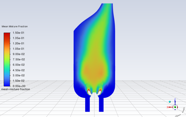
Display filled contours of mean mixture fraction on the surface plane_xz (Figure 18.7: Contours of Mean Mixture Fraction).
Results → Graphics → Contours → New...
1. Enter mean-mixture-fraction for Contour Name.
2. From the Contours of drop-down lists, select Pdf... and Mean Mixture Fraction.
3. From the Surfaces selection list, deselect all surfaces and select plane_xz.
4. Enable Filled in the Options group box.
5. Clear the Auto Range and Clip to Range options.
6. Enter 0.15 for Max.
7. In the Coloring group box, select Smooth.
8. Click Save/Display.
  Figure 18.7: Contours of Mean Mixture Fraction
Display filled contours of CO₂ mass fraction in the combustion chamber (Figure 18.8: Contours of CO₂ Mass Fraction).
Results → Graphics → Contours → co2-mass-fraction Display
Figure 18.8: Contours of CO₂ Mass Fraction

The steady diffusion flamelet simulation yields a significantly different CO₂ mass fraction distribution as compared to the eddy dissipation model calculation. The lower CO₂ concentration at the base of the flamelet flame is caused by low local temperature in the area, which results in slower combustion. In the eddy dissipation model, chemical kinetics is ignored, and the reaction is controlled by turbulent mixing of the materials. In this case, the CO₂ concentration is greater near the base of the flame because the rate of mixing is high in the area (see Figure 18.4: Contours of CO₂ Mass Fraction).
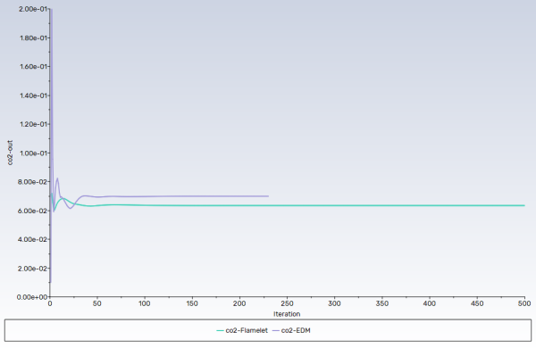
Display the outlet CO₂ concentration profiles for both solutions on a single plot.
Results → Plots → Data Sources...
1. In the Plot Data Sources dialog box, click the Load File... button to open the Select File dialog box.
2. In the Select File dialog box that opens, click once on co2-out-fl-rfile.out and co2-out-rfile.out.
  Each of these files will be listed with their folder path in the bottom list to indicate that they have been selected.
  
  Tip: If you select a file by mistake, simply click the file in the bottom list and then click Remove.
3. Click OK to save the files and close the Select File dialog box.
4. In the Plot group box, enter co2-out for Title.
5. From the Curve Information selection list, select co2-out-rfile.out | Iteration | co2-out
6. Enter co2-EDM in the lower-right text-entry box under the Legend Names selection list.
7. Click the Change Legend Entry button.
  The item in the Legend Entries list for co2-out-rfile.out | Iteration | co2-out will be changed to co2-EDM. This legend entry will be displayed in the upper-left corner of the XY plot generated in a later step.
8. In a similar manner, change the legend entry for the co2-out-fl-rfile.out | Iteration | co2-out curve to be co2-Flamelet.
9. Click the Axes... button to open the Axes dialog box.
  1. From the Axis list, select Y.
  2. Enter 2 for Precision.
  3. Click Apply and close the Axes dialog box.
10. Click the Curves... button to open the Curves dialog box, where you will define a different curve symbol for the CO₂ concentration data.
  1. Retain 0 for the Curve #.
  2. Select ---- from the Pattern drop-down list.
  3. From the Symbol drop-down list, select the "blank" choice, which is the first item in the Symbol list.
  4. Click Apply.
  5. Set Curve # to 1 by clicking the up-arrow button.
  6. Modify the settings for Pattern and Symbol in a manner similar to that for the previous curve.
  7. Click Apply and close the Curves dialog box.
11. Click Plot and close the Plot Data Sources dialog box.
  Figure 18.9: Convergence History of Mass-Weighted Average CO₂ on the Outlet
  
  Despite the model differences, both models predicted similar mass-weighted average mass fractions of CO₂ exiting the combustor during the steady-state. However, the steady diffusion flamelet model predicts less CO₂ exiting the combustor and, due to its more realistic description of combustion kinetics, is considered to be more accurate.
Save the case file (can_combustor_flamelet.cas.h5).
File → Write → Case...

You can perform further postprocessing of the solution results as shown in the following video:

18.6. Summary

In this tutorial, you have learned how to model the reacting flow through a can combustor using the eddy dissipation model and steady diffusion flamelet model in Ansys Fluent.