Chapter 6: Exhaust System: Fault-tolerant Meshing

This tutorial is divided into the following sections:

6.1. Introduction

This tutorial illustrates the setup and solution of a three-dimensional turbulent fluid flow in a manifold exhaust system. The manifold configuration is encountered in the automotive industry. It is often important to predict the flow field in the area of the mixing region in order to properly design the junction. You will use the Fault-tolerant Meshing guided workflow, which unlike the watertight workflow used in Fluid Flow in an Exhaust Manifold, is appropriate for geometries with imperfections, such as gaps and leakages.

This tutorial demonstrates how to do the following in Ansys Fluent:

Use the Fault-tolerant Meshing guided workflow to:
- Import a CAD geometry and manage individual parts
- Generate a surface mesh
- Cap inlets and outlets
- Extract a fluid region
- Define leakages
- Extract edge features
- Setup size controls
- Generate a volume mesh
Set up appropriate physics and boundary conditions.
Calculate a solution.
Review the results of the simulation.

Related video that demonstrates steps for setting up, solving, and postprocessing the solution results for a turbulent flow within a manifold:

6.2. Prerequisites

This tutorial is written with the assumption that you have completed the introductory tutorials found in this manual and that you are familiar with the Ansys Fluent outline view and ribbon structure. Some steps in the setup and solution procedure will not be shown explicitly.

6.3. Problem Description

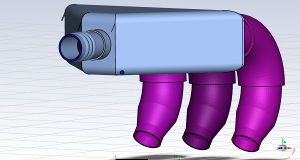
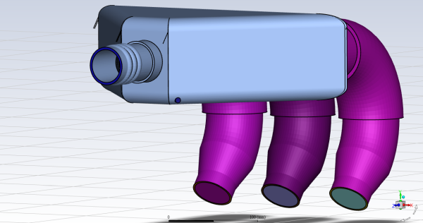
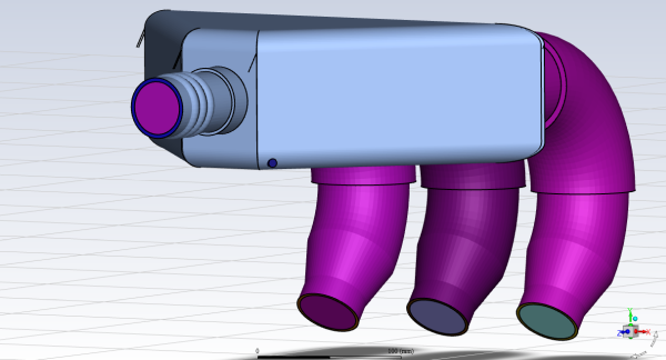
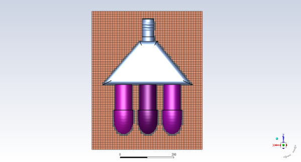
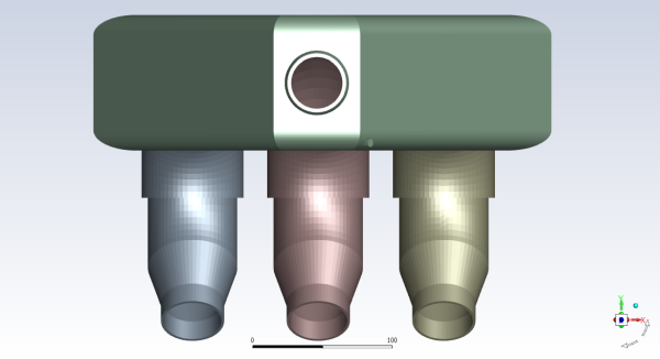
The manifold modeled here is shown in Figure 6.1: Exhaust System Geometry for Flow Modeling. Air flows through the three inlets with a uniform velocity of 1 m/s, and then exits through the outlet.

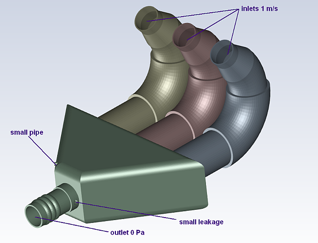
Figure 6.1: Exhaust System Geometry for Flow Modeling

A small pipe is placed in the main portion of the manifold where edge extraction will be considered. There is also a known small leakage included that will be addressed in the meshing portion of the tutorial to demonstrate the automatic leakage detection aspects of the meshing workflow.

6.4. Setup and Solution

The following sections describe the setup and solution steps for this tutorial:

6.4.1. Preparation

To prepare for running this tutorial:

Download the exhaust_system.zip file here .
Unzip exhaust_system.zip to your working directory.
The CAD file exhaust_system.fmd can be found in the folder.
Use the Fluent Launcher to start Ansys Fluent.
Select Meshing in the top-left selection list to start Fluent in Meshing Mode.
Enable Double Precision under Options.
Set Meshing Processes and Solver Processes to 4 under Parallel (Local Machine).

6.4.2. Geometry and Mesh

In this step, we will use Ansys Fluent's guided workflow to import a CAD geometry, and perform various enhancements so that we can generate a complete surface and volume mesh for a complete CFD analysis.

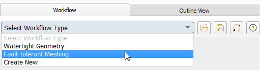
Start the Fault-tolerant Meshing workflow.
1. In the Workflow tab, select the Fault-tolerant Meshing workflow.
2. Review the tasks of the workflow.
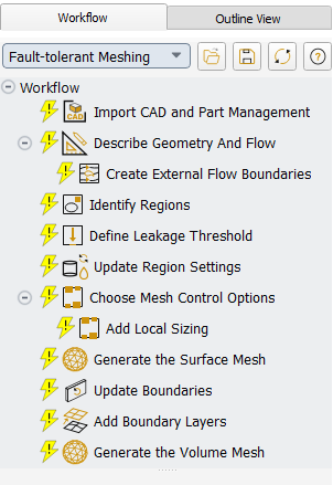
  Each task is designated with an icon indicating its state (for example, as complete, incomplete, etc. All tasks are initially incomplete and you proceed through the workflow completing all tasks. Additional tasks are also available for the workflow.
Import the CAD geometry (exhaust_system.fmd).
1. Select the Import CAD and Part Management task.
2. For CAD File, enter the path and file name for the CAD geometry that you want to import (exhaust_system.fmd).
3. Perform some selective part management.
  1. Select Custom for Create Meshing Objects.
    Using the Custom option allows you load the CAD objects, and selectively pick and choose which parts you want to include in your CFD simulation as meshing objects. Selecting the One per part option would load the CAD geometry and automatically create meshing objects for every part.
  2. For Display Unit, keep the default setting as mm.
  3. Click the Load button.
    This will load the CAD file's content into the CAD Model tree below.
    
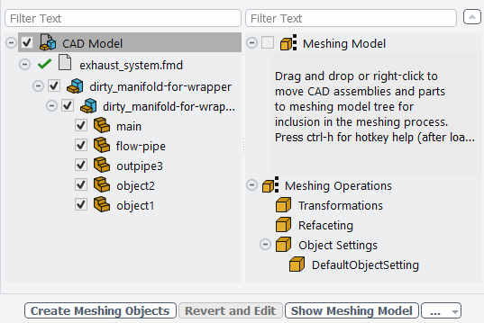
    Note: Items in the model trees that are checked indicate an object that is displayed in the graphics window. Using the check boxes is not the same as selecting a object in the tree to perform a particular operation.
    Figure 6.2: Manifold CAD Geometry for Flow Modeling
  4. In the CAD Model tree, select the first part (main), hold the Shift button and select the last part (object1), thereby selecting all of the parts.
    You can also select the parts you require in the graphics window.
  5. Holding down the left mouse button, drag the collection of parts and drop them onto the Meshing Model tree.
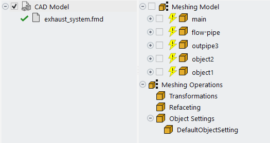
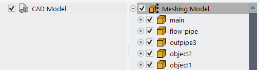
    The parts in the CAD Model tree will become grayed out and will appear in the Meshing Model tree. If you make a mistake, you can right-click the appropriate node in the Meshing Model tree, and select the Restore to Cad Model option from the context menu, and the parts will be restored to the CAD Model tree.
    Note: You can also select objects in the graphics window and add them to the tree.
    Make sure that you select the check box for the top-level node in the Meshing Model tree to view all of the parts of the meshing model in the graphics window.
4. Click Create Meshing Objects at the bottom of the task.
  This will update the task, create meshing objects with the designated properties based on the selected portions of the CAD model. This will also display the geometry in the graphics window, and allow you to proceed onto the next task in the workflow.
  Throughout the workflow, you are able to return to a task and change its settings using either the Edit button, or the Revert and Edit button.
Provide a description for the geometry and the flow characteristics.
1. In the Describe Geometry and Flow task, you are prompted for more information about the geometry and flow.
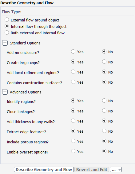
2. Select Internal flow through the object for the Flow Type.
3. Enable Advanced Options to expose additional options that are required for this task.
  Many workflow tasks have advanced options that you may want to inspect before updating a task.
4. Select Yes for the Extract edge features? prompt.
  This particular geometry has a few areas that will require special feature extraction treatment.
5. Click Describe Geometry and Flow to complete this task and proceed to the next task in the workflow.
Cover any openings in your geometry.
Select the Enclose Fluid Regions (Capping) task, where you can cover, or cap, any openings in your geometry in order to later extract the enclosed fluid region.
1. Create a cap for one of the inlets.
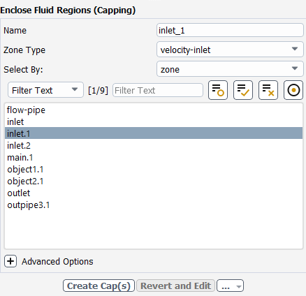
  1. In the Name field, enter inlet_1 for the name of the capping surface to be applied to one of the manifold's inlets.
  2. For the Zone Type field, choose velocity-inlet.
  3. For the Select By field, choose zone.
  4. In the list of zones, select inlet.1 as the opening that you want to cover.
    For occasions when the list of items is long, you can use the Filter Text option and use an expression such as in* to show only items starting with "in". Alternatively, you can use the Use Wildcard option to list and pres-select matching items. See Filtering Lists and Using Wildcards for more information.
    The graphics window indicates the selected item.
  5. Click Create Cap(s) to complete this task and proceed to the next task in the workflow.
    Once completed, this particular task will return you to a fresh task in order to assign additional capping surfaces, if necessary. We will proceed to assign a cap for the remaining openings.
2. Repeat the previous steps, creating a cap called inlet_2 for the inlet.2 zone, and another cap called inlet_3 for the inlet zone.
  This will cover all of the manifold's inlets.
  Alternatively, you could also have selected all three inlet zones and created a single cap for all three inlets.
3. Create a cap for the outlet.
  1. In the Name field, enter outlet_1 for the name of the capping surface to be applied to the manifold's outlet.
  2. For the Zone Type field, choose pressure-outlet.
  3. For the Select By field, specify zone.
  4. In the list of zones, select outlet for the outlet that you want to cover.
  5. Click Create Cap(s) to complete this task.
  Now, all of the openings in the geometry are covered.
Extract edge features.
In the Extract Edge Features task, you can set various properties for the extraction of features in your geometry.
In this tutorial, we will create a single extraction object to capture the features between the smaller pipe and the main manifold.
Create a feature extraction object based on intersection loops between the smaller pipe and the main manifold.
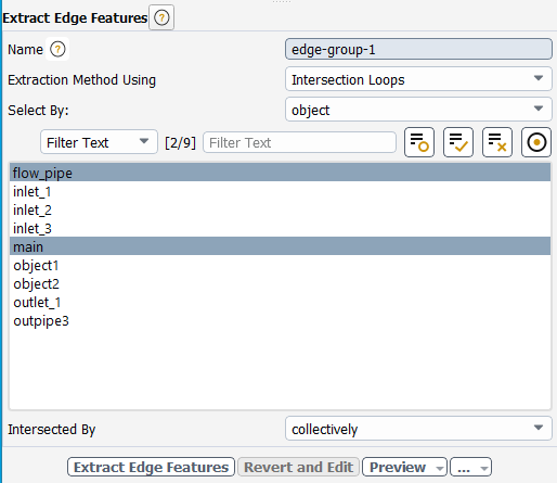
1. Keep the default Name as edge-group-1
2. Select Intersection Loops for the Extraction Method Using field.
3. Select main and flow_pipe in the Objects list.
4. Keep the default Intersected By setting as collectively.
  This will localize the feature extraction to the intersection of the small pipe (flow_pipe) with the main manifold (main).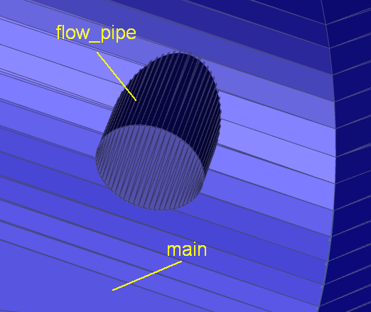
5. Click Extract Edge Features to complete this task and proceed to the next task in the workflow.
Identify regions.
In the Identify Regions task, you can choose the various regions that you want to use in your simulation.
In this tutorial, we will identify the internal fluid region as well as the external (void) region outside of the geometry. The external void region will be useful in identifying any potential leakages from within the fluid region to the outer domain.
1. Identify the fluid region.
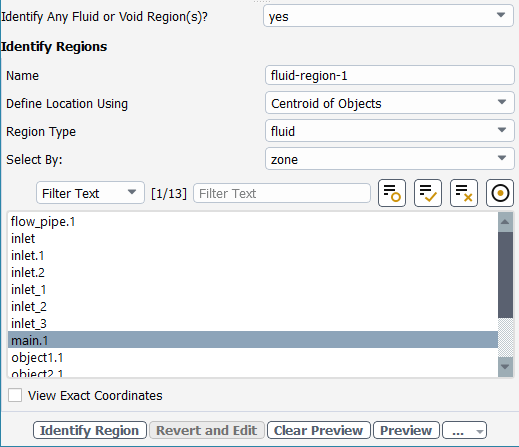
  1. For the Identify any fluid or void region(s)? prompt, keep the default setting of yes.
  2. Keep the default Name as fluid-region-1
  3. Keep the default Define Location Using setting as Centroid of Objects.
  4. Keep the default Region Type setting as fluid.
  5. Set the Select By setting to zone.
  6. Select main.1 in the list of zones.
  7. Click Identify Region.
    Once completed, this particular task will return you to a fresh task in order to identify additional regions, if necessary. We will proceed to identify a void region.
2. Identify the region outside the geometry.
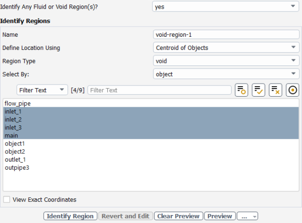
  1. Change the Region Type setting to void.
  2. Keep the default Name as void-region-1
  3. Keep the default Define Location Using setting as Centroid of Objects.
  4. Keep the default Select By setting as object.
  5. Select main, inlet_1, inlet_2, and inlet_3 in the list of objects.
    This will ensure that the void region is located properly based on the centroid of the selected objects.
  6. Click Identify Region to complete this task and proceed to the next task in the workflow.
Define thresholds for any potential leakages.
In the Define Leakage Threshold task, you can choose to define a threshold for when leakages within your geometry can be identified and automatically patched.
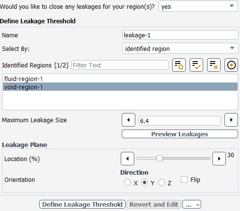
1. Specify yes at the prompt to define a leakage threshold.
  In the case of this tutorial, we know there is a potential leakage (a small opening in the main manifold in the neck of the outlet) that we want to define a threshold.
2. Keep the default Name as leakage-1
3. Keep the default Select By: as identified region
4. Select void-region-1 from the Regions list.
5. Keep the default value of 6.4 mm for the Maximum Leakage Size.
6. Click Preview Leakages.
  This will display a cut plane through the domain that you can adjust using the Leakage Plane controls. Use the Location slider and the Orientation fields to identify any potential leakages with the current settings.
7. Adjust the Location slider to a value of 30 mm.
8. Change the Orientation setting to Y.
  Rotate the display and examine the mesh. Note that there are no leakages present.
9. Click Define Leakage Threshold to complete this task and proceed to the next task in the workflow.
Review your region settings.
1. In the Update Region Settings task, you can review and revise a table of settings for the defined regions.
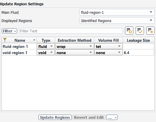
2. For the Displayed Regions field, select Identified Regions, as a means of simplifying the listing to only show previously identified regions.
3. For fluid-region-1, change the Volume Fill setting from hexcore to tet, since, for internal flow, we are interested only in using tetrahedral cells.
  To change the setting in the table, double-click the cell to expose the drop-down menu options.
4. Keep the Volume Fill setting for void-region-1 set to none.
  This is done since we do not want to consider the void region, however, we want to use the Leakage Size threshold of 6.4 mm to detect any leakages from the fluid region into the void region when that threshold is exceeded.
5. Click Update Regions to complete this task and proceed to the next task in the workflow.
Select options for controlling the mesh.
In the Choose Mesh Control Options task, you can determine how much control you want when generating the mesh: either through size controls; and/or through boundary layer settings.
For the purposes of this tutorial, you can keep the default settings in this task.

Click Choose Options.
This will create a Add Local Sizing task.
1. For the Add Local Sizing task, keep the default size controls (default-curvature and default-proximity) already populated with useful default settings.
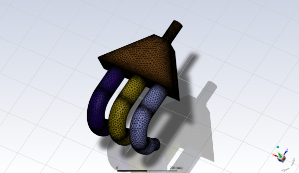
Generate the surface mesh.
1. In the Generate the Surface Mesh task, you can customize how the surface mesh is created.
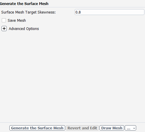
2. Click Generate the Surface Mesh to complete this task and proceed to the next task in the workflow.
  Ansys Fluent will apply your settings (calculate size fields, closing leakages, remeshing surfaces, calculating regions, etc.) and proceed to generate a surface mesh for the manifold geometry. You can visualize the surface mesh by selecting the Draw Mesh button at the bottom of the task, and adjusting the clipping plane controls accordingly.
Confirm and update the boundaries.
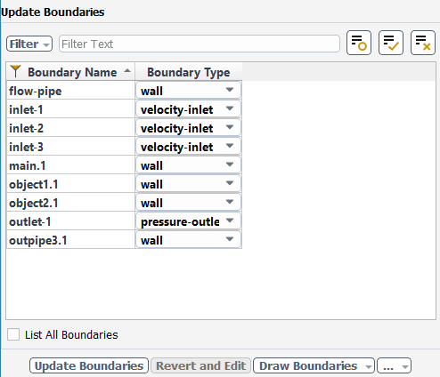
1. Select the Update Boundaries task, where you can inspect the mesh boundaries and confirm and change any designated boundaries accordingly. Ansys Fluent attempts to determine the correct arrangement of boundaries automatically.
2. All the proposed boundaries are correct, so click Update Boundaries. and proceed to the next task.
Add boundary layers.
For the Add Boundary Layers task, select yes at the prompt as to whether or not you want to define boundary layer settings. In this task, you can define specific details for capturing the boundary layer in and around your geometry.
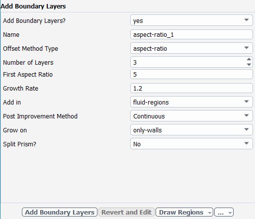
1. Select Continuous from the Post Improvement Method list.
  These default settings create a continuous boundary layer along the walls of the fluid region.
2. Click Add Boundary Layers to complete this task and proceed to the next task in the workflow.
Generate the volume mesh.
1. In the Generate the Volume Mesh task, you can customize how the volume mesh is created, primarily defining the final skewness for the volume mesh.
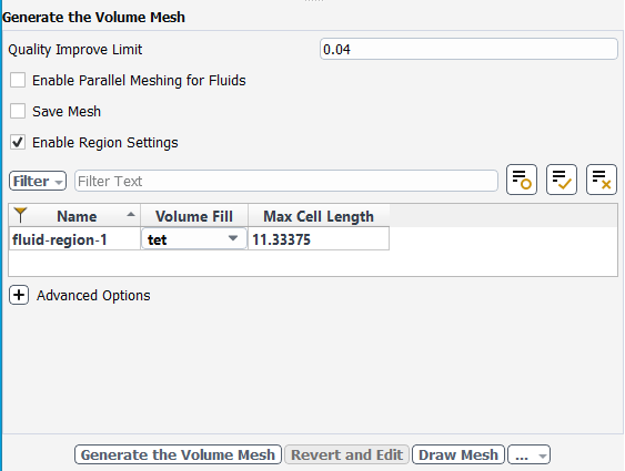
2. Select the Enable Region Settings to view and edit volume fill settings, prior to actually generating the fluid volume mesh.
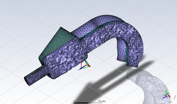
3. Click Generate the Volume Mesh to complete this task and proceed to the next task in the workflow.
  Ansys Fluent will apply your settings and proceed to generate a volume mesh for the manifold geometry. Once complete, the mesh is displayed in the graphics window and a clipping plane is automatically inserted with a layer of cells drawn so that you can quickly see the details of the volume mesh.
Check the mesh.
Mesh → Check → Perform Mesh Check
Save the mesh file (exhaust_system.msh.h5).
File → Write → Mesh...
Switch to Solution mode.
Now that a high-quality mesh has been generated using Ansys Fluent in meshing mode, you can now switch to solver mode to complete the set up of the simulation.
We have just checked the mesh, so select Yes when prompted to switch to solution mode.

6.4.3. General Settings

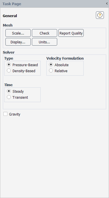
In the Mesh group box of the Domain ribbon tab, set the units for length.

Domain → Mesh → Units...

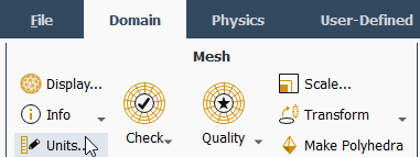
This opens the Set Units dialog box.

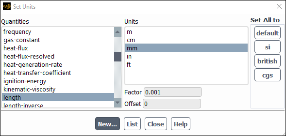
Select length under Quantities.
Select mm under Units.
Close the Set Units dialog box.

6.4.4. Solver Settings

In the Solver group box of the Physics ribbon tab, retain the default selection of the steady pressure-based solver.

Physics → Solver

6.4.5. Models

Set up your models for the CFD simulation using the Models group box of the Physics ribbon tab.

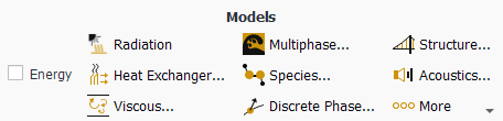
Note: You can also use the Models task page, which can be accessed from the tree by expanding Setup and double-clicking the Models tree item.
Retain the default k-ω SST turbulence model.
You will use the default settings for the k-ω SST turbulence model, so you can enable it directly from the tree by right-clicking the Viscous node and choosing SST k-omega from the context menu.
Setup → Models → Viscous Model → SST k-omega

6.4.6. Materials

Ordinarily, you would set up the materials for the CFD simulation using the Materials group box of the Physics ribbon tab.

In this tutorial, we will keep the default fluid material of air.

6.4.7. Cell Zone Conditions

Ordinarily, you would set up the cell zone conditions for the CFD simulation using the Zones group box of the Physics ribbon tab.

In this tutorial, we will keep the default assignment of air for the fluid zone.

6.4.8. Boundary Conditions

Set the velocity and turbulence boundary conditions for the first inlet (inlet-1).
Setup → Boundary Conditions → Inlet → inlet_1 Edit...
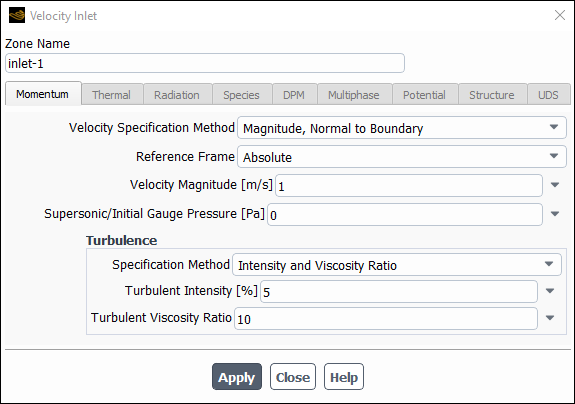
1. Enter 1 m/s for Velocity Magnitude.
2. Keep the remaining default settings.
3. Click Apply and close the Velocity Inlet dialog box.
Apply the same conditions for the other velocity inlet boundaries (inlet_2, and inlet_3).
Set the boundary conditions at the outlet (outlet-1).
Setup → Boundary Conditions → Outlet → outlet_1 Edit...
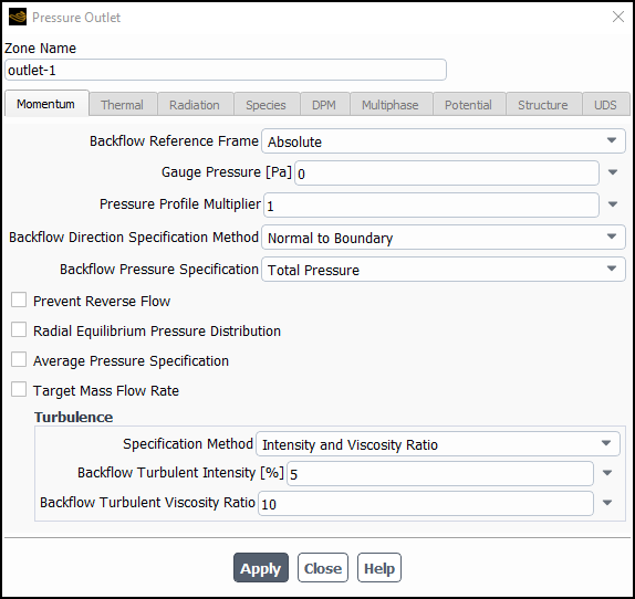
1. Retain the default setting of 0 for Gauge Pressure.
2. Keep the remaining default settings.
3. Click Apply and close the Pressure Outlet dialog box.
Retain the remaining default (wall and interior) boundary conditions.

6.4.9. Solution

Specify the discretization schemes.
In the Solution ribbon tab, click Methods... (Solution group box).
Solution → Solution → Methods...
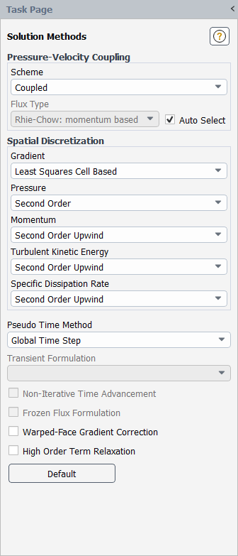
1. Retain the default settings for Solution Methods.
Monitor the mass flow rate at the inlets.
Solution → Reports → Definitions → New → Flux Report → Mass Flow Rate...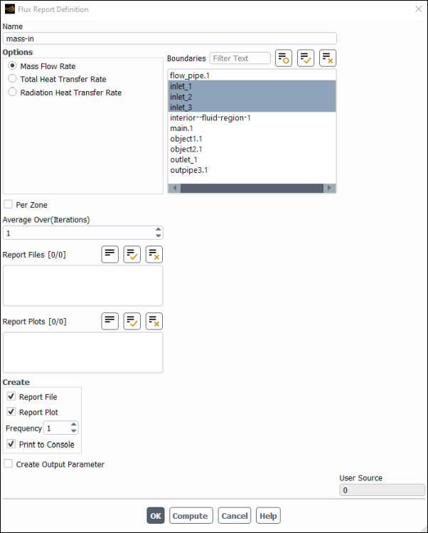
1. Enter mass-in for the Name of the report definition.
2. Ensure Mass Flow Rate is selected in the Options group box.
3. Select inlet_1, inlet_2, and inlet_3, from the Boundaries selection list.
4. Enable Report Plot and Print to Console in the Create group box.
5. Click OK to save the surface report definition and close the Flux Report Definition dialog box.
Monitor the total mass flow rate through the entire domain.
Perform the same procedure as described above, naming the report mass-tot, and selecting the boundaries inlet_1, inlet_2, inlet_3, and outlet_1.
Monitor the mass balance.
Solution → Reports → Definitions → New → Expression...
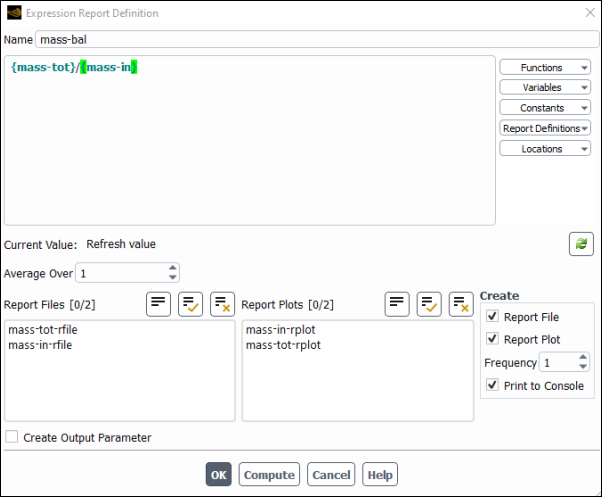
1. Enter mass-bal for the Name of the expression.
2. Select mass-tot from the Report Definitions drop-down list on the right.
3. Type the / operand.
4. Select mass-in from the Report Definitions drop-down list on the right.
5. Enable Report Plot and Print to Console in the Create group box.
6. Click OK to save the expression definition.
Initialize the flow field using the Initialization group box of the Solution ribbon tab.
Solution → Initialization
1. Select Standard from the Method list.
2. Click Initialize.
Save the case file (exhaust_system.cas.h5).
File → Write → Case...
Start the calculation by requesting 100 iterations in the Solution ribbon tab (Run Calculation group box).
Solution → Run Calculation
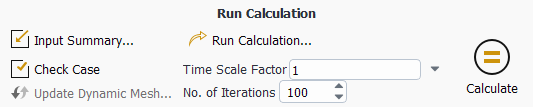
1. Enter 100 for No. of Iterations.
2. Click Calculate to begin the iterations.
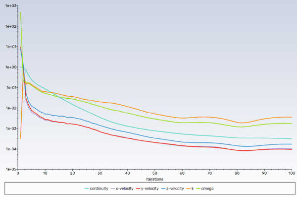
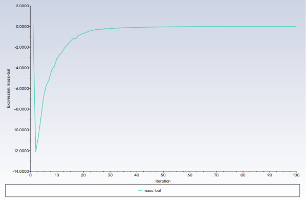
  As the solution progresses, the residuals history will be plotted in the Scaled Residuals tab in the graphics window (Figure 6.3: Residuals).
  Figure 6.3: Residuals
3. Similarly, the monitors will be plotted in their respective tabs in the graphics window.
  Figure 6.4: Mass Balance History
  
  The net mass imbalance is a small fraction (less than 0.5%) of the total mass flow rate through the system, which indicates that the solution has converged.
Save the case and data files (exhaust_system.cas.h5 and exhaust_system.dat.h5).
File → Write → Case & Data...

6.4.10. Postprocessing

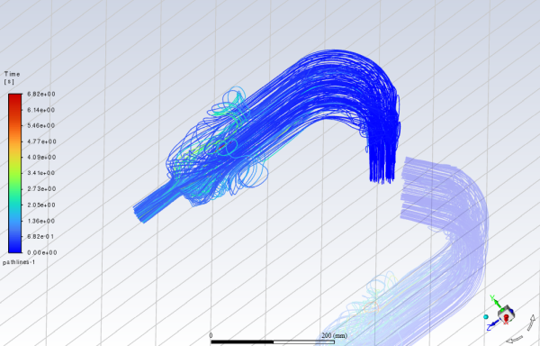
Display path lines highlighting the flow field (Figure 6.5: Pathlines Through the Manifold).
Results → Graphics → Pathlines → New...
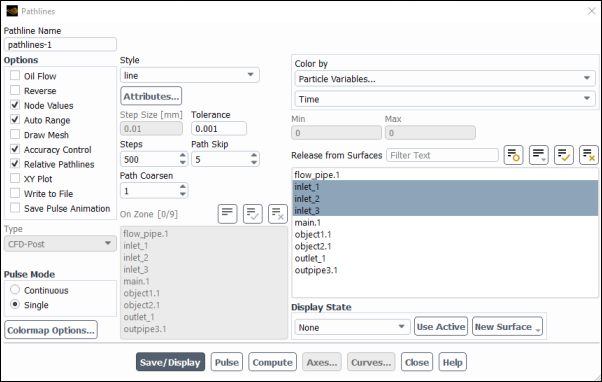
1. Keep the default of pathlines-1 for the Name.
2. Select Particle Variables... and Time from the Color by drop-down lists.
3. Enable Accuracy Control under Options.
4. Set the Path Skip value to 5.
5. Select inlet-1, inlet-2, and inlet-3 from the Release from Surfaces list.
6. Click Save/Display and close the Pathlines dialog box.
  The new pathlines-1 definition appears under the Results/Graphics/Pathlines tree branch. To edit your surface definition, right-click it and select Edit... from the menu that opens.
  Figure 6.5: Pathlines Through the Manifold
Create an iso-surface through the manifold geometry.
Results → Surface → Create → Iso-Surface...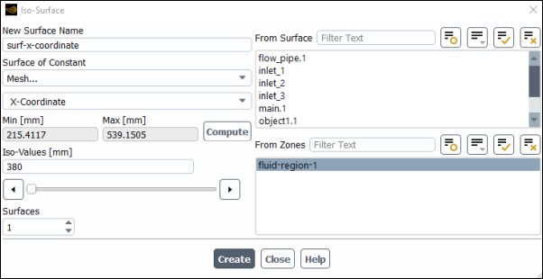
1. Select Mesh... and X-Coordinate from the Surface of Constant drop-down lists.
2. Enter surf-x-coordinate for the Name.
3. Select fluid-region-1 from the From Zones list.
4. Click Compute.
5. Use the slider to locate the iso-surface in the middle of the geometry (approximately 380 mm).
6. Click Create and close the Iso-Surface dialog box.
  The new surf-x-coordinate definition appears under the Results/Surfaces tree branch. To edit your surface definition, right-click it and select Edit... from the menu that opens.
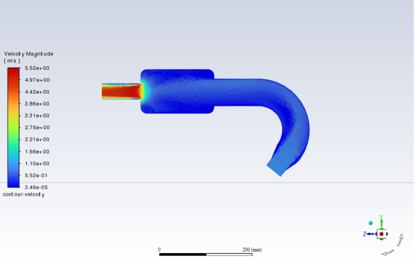
Create and define contours of velocity magnitude throughout the manifold along with the mesh.
Results → Graphics → Contours → New...
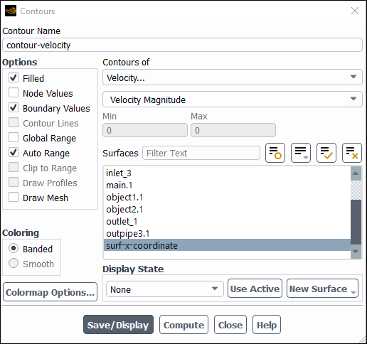
1. Enter contour-velocity for the Name.
2. Select Velocity... and Velocity Magnitude from the Contours of drop-down lists.
3. Select surf-x-coordinate from the Surfaces list.
4. Disable Node Values under Options.
5. Disable Global Range under Options.
6. Click Save/Display and close the Contours dialog box.
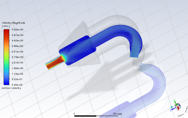
Figure 6.6: Contours of Velocity Magnitude Through the Manifold
Create a scene containing the mesh and the contours.
Results → Scene New...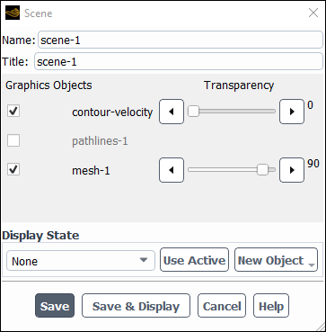
1. Keep the default scene-1 for the Name and Title.
2. Select contour-velocity under Graphical Objects.
3. Create a new mesh object to add to the scene.
  1. Click New Object and select Mesh to open the Mesh Display dialog box.
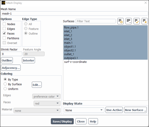
  2. Select all of the surfaces under the Surfaces list, except the newly created surface.
  3. Click Save/Display and close the Mesh Display dialog box.
    The new mesh-1 definition appears under the Results/Graphics/Mesh tree branch. The new object also appears in the Scene dialog box.
4. In the Scene dialog box, set the Transparency to 90 for the mesh-1 graphical object.
5. Click Save & Display and close the Scene dialog box.
  Figure 6.7: Scene Containing the Mesh and Contours Throughout the Manifold
6. Save the case file (exhaust_system.cas.h5).
  File → Write → Case...

6.5. Summary

In this tutorial, you learned how to import a faulty CAD geometry, add modifications and enhancements, generate a volume mesh, and set up, solve, and postprocess a CFD problem involving air flow through a exhaust system.

Related video that demonstrates steps for setting up, solving, and postprocessing the solution results for a turbulent flow within a manifold: