Exporting ROM Radar to VRXPERIENCE (Beta)

The VRXPERIENCE Sensors simulation environment includes a ROM-based automotive radar model based on the Ansys FF-RRP ROM (Far-Field Rotated Range Profile Reduced Order Model). This ROM is generated by HFSS SBR+. It consists of coherent radar cross-section (RCS) data of a radar target (e.g., car, truck, infrastructure) collected over a range of frequencies and aspect angles. The RCS data are captured in four polarization combinations: VV, HV, VH, and HH. The frequency sweep is typically broad enough to cover the range of frequencies permitted in a particular automotive radar band (e.g., 76 - 81 GHz). VRXPERIENCE Sensors can ingest multiple ROM files to simulate complex traffic engagements in real time. Details and instructions for using HFSS-exported FF-RRP ROM files in VRXPERIENCE Sensors can be found in its end-user documentation. This help page describes the HFSS work flow for synthesizing and exporting an FF-RRP ROM file for a single radar target.

Prerequisites

Requirements for generating a FF-RRP ROM file:

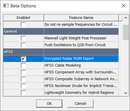
• Use Tools>Options>General Options to open Options dialog box, and under Desktop Configuration, select the Beta Options button, enable Encrypted Radar ROM Export. You will need to restart Ansys Electronics Desktop to use the enabled Beta Options.

• A CAD model for the radar target. Alternatively, the model can be drawn in HFSS.
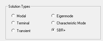
• Solution type must be SBR+.
• Bounds for the intended radar frequency band. For example, based on international standards, the 77-GHz automotive radar band extends from 76 to 81 GHz. To maximize their generality of application, FF-RRP ROM files intended for simulating “77-GHz” automotive radars should use a frequency sweep from 76 to 81 GHz. The fact that a particular radar only uses a portion of the 76 – 81 GHz band should not weigh in setting the frequency sweep of an FF-RRP ROM file, as that would block its use with other radars that operate in a different portion of that band. At the same time, it is not recommended to create an FF-RRP ROM file that spans the 24-GHz and 77-GHz automotive radar bands since that results in immense wasted computation and storage covering the large gap between these band where no automotive radars operate.

Synthesizing and Exporting an FF-RRP ROM File

1. Create an HFSS design and set its Solution Type to SBR+.

Right-click on the HFSS design node in the Project tree and select Solution Type… . In the dialog that appears, select SBR+ and then OK.

Note: The other HFSS solution types do not support generating a ROM file.

2. Import the CAD model(s) representing the radar target.

CAD models in various formats can be imported via Modeler> Import…. If the target is to be assembled from multiple parts, be sure they are properly arranged relative to each other and then group them together before proceeding to the next step.

3. Position and orient the radar target.

Perform Move and Rotate operations on the target geometry model so that it is positioned and oriented correctly in HFSS global coordinates. It is important that vehicles be positioned and oriented as follows in HFSS global coordinates:

• X-, Y-, and Z-axis point out the front, right side, and top of the vehicle, respectively
• Bottom of wheels touch XY-plane at Z = 0
• Vehicle bounding box extends from (-L/2,-W/2,0) to (L/2,W/2,H):

L = length, W = width, H = height .

Laterally centering the vehicle about the origin of the XY-plane minimizes the opportunity for range aliasing in range-Doppler imagery generated by the VRXPERIENCE ROM-based radar sensor model.

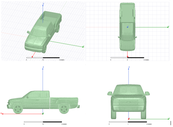
Note: It is important that HFSS and VRXPERIENCE Sensors use an identical or nearly identical CAD model for visualization and identical local coordinate systems for the target.

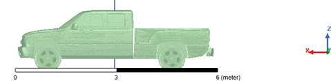
In preparation for later configuring the density of the frequency sweep in the solution setup, determine the longest dimension D of the radar target. This can be done by aligning the target with the ruler at the bottom of the display or by using the Measure tool found in the Draw ribbon. It is not important to measure D with great precision, but in that case, one should err on the high side. In the truck example illustrated below, D = 6.0 m.

4. Apply boundary assignments to the surfaces.

Since this is an SBR+ simulation, material properties of the radar target should be configured via boundary assignments, not volumetric material assignments. In the absence of better information, the entire vehicle can be configured as Perfect E. Fidelity can be improved by investing the effort to assign more realistic boundaries, particularly for glass windows, tires, and exterior plastic/rubber. The following types of boundary assignments are recommended:

Perfect E: Metal surfaces of body.

Layered Impedance (one-sided): Tire rubber, body plastic, mirrors, interior seats. Can also be used for painted metal surfaces to improve fidelity. One-sided Layered Impedance boundaries only reflect SBR rays; they generate no transmission rays.

Layered Impedance (two-sided): glass windows. Two-sided layered impedance boundaries are penetrable to rays. For this reason, they can also be used for things like non-metallic bumpers provided the vehicle structure underneath these covering surfaces is adequately captured in the CAD model. Barring that, it is recommended to model non-metallic exterior parts using one-sided Layered Impedance boundaries. When using two-sided Layered Impedance boundaries for things like windows, they should be represented by a single thin sheet in the CAD model, not a closed volumetric object nor a pair of sheets to represent the inside and outside surfaces. The finite thickness of the glass should be captured in the assigned thicknesses of the window layer(s) in the Layered Impedance boundary configuration. Also, be careful when applying two-sided Layered Impedance boundaries to the face(s) of a closed object (as opposed to a sheet). The object volume material must be set to vacuum, and it should be understood that each SBR ray will branch into a transmission and reflection ray upon hitting the object face, whether incident from the outside or (later) incident from the inside after a transmission rays has penetrated into the object. As a result, many rays will repeatedly bounce inside the closed object volume until reaching the Maximum Number of Bounces limit. In special cases, such a configuration can make sense for some components, but if the closed object volume is not actually vacuum (or air filled), this would be the incorrect way to model it and one should instead fall back on applying a one-sided Layer Impedance boundary to all faces of the object and setting the infinite-thickness layer to the dielectric properties of the volume object.

Perfect Absorber: When the CAD model has gaps, making it leaky to rays, adding Fresnel SBR+ Perfect Absorber surfaces to the interior of the target is a good way to trap rays that leak inside and prevent them from rattling around the interior, which would tend to harm accuracy.

5. Create a pair of incident plane-wave excitations with an angular sweep, one for vertical polarization and one for horizontal polarization.

The ROM model content is coherent, monostatic RCS in four polarization combinations that provide a complete polarimetric description of the scattering: VV, HV, VH, and HH. There are two independent incident polarizations (indicated by the second letter), and for each of these there are two independent observation polarizations (indicated by the first letter).

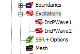
In following steps, the polarization ordering of the two incident plane-wave excitations is interchangeable without affecting the content or data ordering in the ROM file. Also, the default excitation names of IncPWave1 and IncPWave2 are not important and can be changed if desired.

First, configure the incident plane-wave with horizontal polarization:

1. In the Project tree, right-click on the Excitations node and select Assign Incident Wave>Plane Wave….
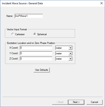
2. In the Incident Wave Source: General Data dialog that appears, set the Vector Input Format to Spherical. As a clarification for post processing, you may want to change the default name to something like IncPlaneWave_H for the first wave, and IncPlaneWave_V for the second wave. Then click Next.

3. In the updated dialog box, set IWavePhi Start and Stop to -180 deg and 180 deg for a full circular sweep around the target. The Step size should be set no higher than 1 deg. A lower Step size can be selected to improve resolution, but realize this will lead to a longer HFSS synthesis time and a larger ROM file. Regardless, make sure that the Step size fits evenly into 360 deg. Otherwise, the final IWavePhi sample at +180 deg might be omitted, resulting in an incomplete ROM model and unexpected results when it is used in VRXPERIENCE. Confirm that the final IWavePhi angle sample is +180 deg by selecting View Point List… and scrolling down to the end of the list.

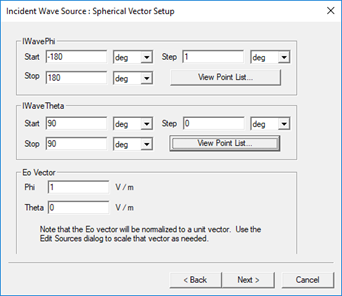
4. In the same dialog box, set IWave Theta Start, Stop, and Step to 90 deg, 90 deg, and 0 deg, respectively. This fixes the elevation angle at zero (0), the XY-plane.
5. In the same dialog box, configure Eo Vector as Phi = 1 V/m, Theta = 0. This sets up a horizontally polarized incident field that yields the VH and HH RCS polarization components.
6. Click Next. In the updated dialog box, accept the default selection (Regular/Propagating) and click Finish. The incident and observation angles of the monostatic RCS sweep have now been configured for HV and HH polarization combinations.
7. To set up the incident vertical polarization, repeat Steps 5a – 5f, but with the following change: in Step 5e, configure Eo Vector as Phi = 0, Theta = 1 V/m. The monostatic RCS sweep for the VV and HV polarization combinations has now also been configured. During simulation, these two incident polarizations will be simulated independently.

6. Create and configure the solution setup.

Create a solution setup that configures a uniform frequency sweep, sets the RCS modality to monostatic (observation angle tracks incident angle), and configures the SBR+ methodology settings.

1. In the Project tree, right-click Analysis and select Add Solution Setup….
2. In the SBR+ Solution Setup dialog that appears, leave the Setup Type as Standard. There will be a table with a single row whose Distribution is set to Linear Step. Left-click on Linear Step and select Linear Count instead.

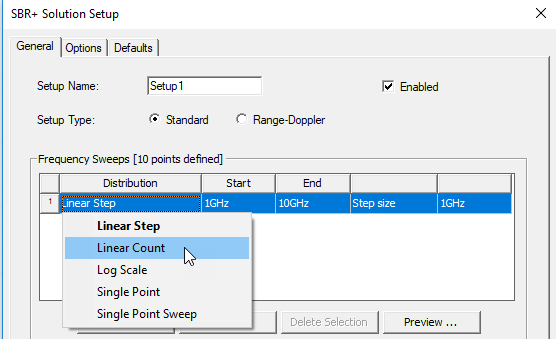
3. Using the longest dimension D of the radar target that was established in Step 3, determine the required frequency interval as Δf = c/6D where, c is the speed of light. Sampling at this frequency (or lower) will minimize the opportunity for range aliasing in radar imagery generated by the ROM-based radar model in VRXPERIENCE Sensors. The above formula includes a safety margin of D behind the vehicle (relative to the radar) for multi-bounce delayed response. In the truck example above, D = 6 m, so Δf = 8.3333 MHz.
4. To generate a ROM model applicable to any automotive radar operating in the 77-GHz band, set the Start and End fields to 76GHz and 81GHz (these are the maximum extents allotted to the 77-GHz automotive radar band). This corresponds to a bandwidth of 5 GHz. Divide the bandwidth by Δf and then round up to obtain an integer number of frequency intervals. Then add one (1) to obtain the number of points and enter this in the far right (unlabeled) field of the table row. In this example, 5 GHz/8.3333 MHz = 600, so enter 601 for the number of points.
5. Make sure that Compute Far Fields is toggled on.
6. Select the Options tab.
   
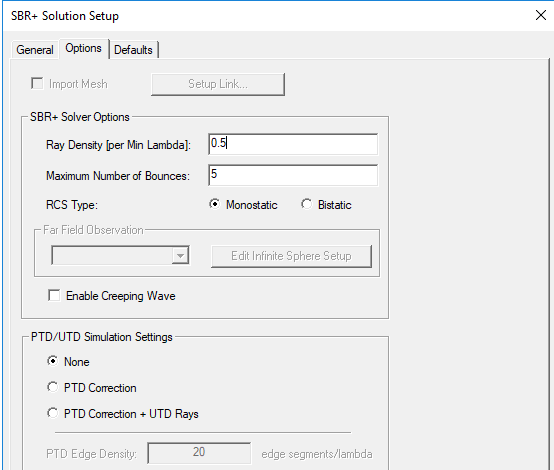
7. Important: Change Ray Density per Min Lamda from its default (4.0) to 0.5. At this nominal 77-GHz frequency, we recommend a setting of 1.0 or less for ray density. Otherwise, far more rays are shot than are really needed, harming simulation time for generating the FF-RRP ROM model (it does not affect dynamic simulation time in VRXPERIENCE Sensors, however).
8. Set RCS Type to Monostatic.
9. Set the Maximum Number of Bounces. The default value of 5 is recommended.
10. If you elect to switch on PTD or PTD + UTD to improve accuracy, you may optionally choose to extract and filter wedges. This can be done by right-clicking SBR+ Options in the Project tree and selecting Wedge Settings….
    

7. Run the simulation (i.e., Analyze the solution setup).

In general, we recommend that you use Ansys HPC to add more cores to speed the solve process.

8. Plot the RCS results (optional).

Generate a plots of RCS vs. angle to verify the results are reasonable.

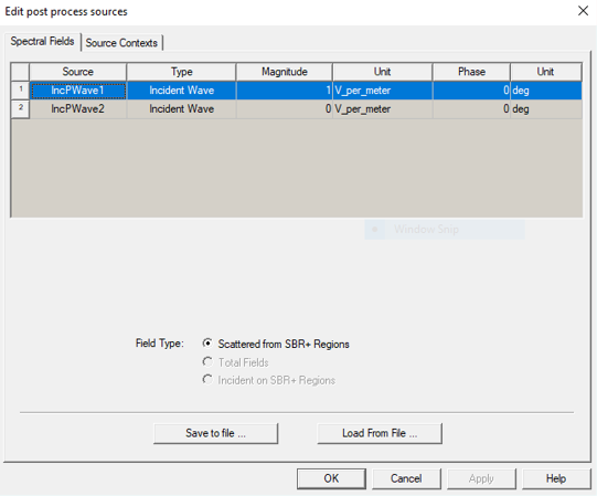
1. Before generating the plot, set/verify the active incident polarization for the plot. In the Project tree, right-click on Excitations and select Edit Sources….
2. In the Edit post process sources dialog that appears, there will be a table with two rows for the two configured plane-wave excitations. If not already configured this way, set Magnitude of IncPWave1 to 1 V/m and that of IncPWave2 to 0 V/m, and then click OK. Since in this example, IncPWave1 was configured as the incident horizontal polarization, any existing or new plot while this edit-sources configuration is active will show results for incident horizontal polarization.

3. In the Project tree, right-click on Reports and select Create Monostatic RCS Report >Rectangular Plot.
4. In the Report dialog box, set Primary Sweep to IWavePhi, under Category select Monostatic RCS, under Quantity select MonostaticRCSPhi, and under Function select dB.

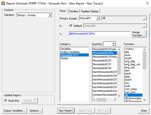
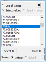
5. Select the Families tab in the same dialog box. This controls the multi-dimensional slicing to configure one or more plot traces. In the table, click the ellipses […] button in the Edit column for the Freq row. This pops up a small dialog for selecting the discrete frequency samples to plot as separate traces. Scroll down, select 77GHz, and close the dialog by clicking the “X” button in its upper right corner.

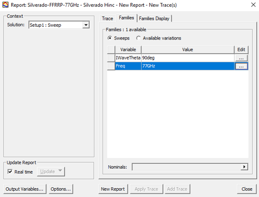
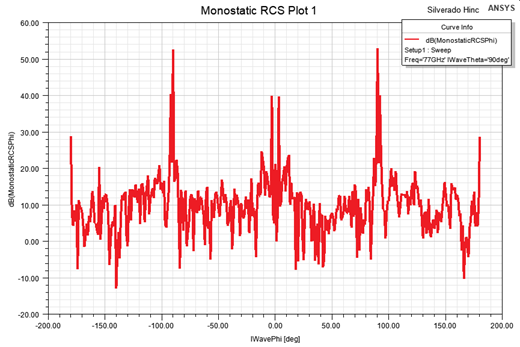
6. At the bottom of the Report dialog box, click New Report. A new plot is created showing the HH-polarization RCS vs. Phi angle at 77 GHz. It is HH polarization because of the combination of the Edit Sources weighting from Step 8b and the Quantity selection from Step 8d. Leave the Report dialog open.

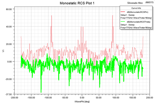
7. In the Report dialog box, select the Trace tab again and then set Quantity to MonostaticRCSTheta. Also make sure to set Function to dB again, then click Add Trace. A second trace is added to the plot that shows the VH-polarization RCS. It is significantly weaker than the HH-polarization, which is typical when comparing cross-polarized to co-polarized RCS.

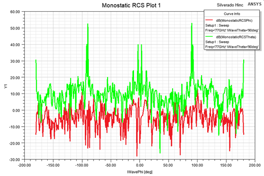
8. Note the sharp peaks at IWavePhi = +/- 180^o and +/- 90^o for the HH-polarization. These are specular flashes off the large and nearly flat surfaces of the back and sides of the truck (in this example). The side flashes are particularly pronounced, exceeding 50 dBsm (dB square-meters) because truck doors and bed walls are nearly perpendicular to the radar and have a very large surface area.

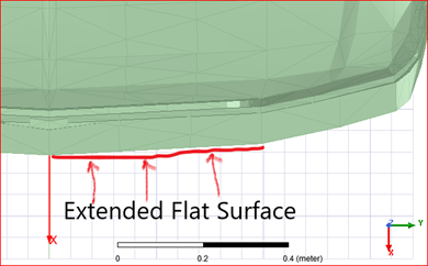
There are also a pair of specular flashes near IWavePhi = +/- 3^o. These are caused by extended flat surfaces on the front bumper and are therefore likely an artifact of the coarse meshing resolution of the bumper. This leads to an important observation: at 77 GHz, the wavelength is approximately 4 mm. Meshings of radar targets that might be perfectly adequate for 10 GHz and below may be too coarse at 77 GHz because flat surfaces of the mesh increase in electrical size, leading to artificial specular flashes. This is likely the situation with the pickup truck model used in this example. The real bumper is a smoothly curved surface, so the observed coarse meshing of the bumper and the correlation of these specular flashes with the angles of the bumper surfaces indicate that it has inadequate mesh resolution for RCS prediction at 77 GHz.

9. Open the Edit Sources dialog again (see Step 8a) and set the Magnitude for IncPWave1 to 0 and IncPWave2 to 1 V/m. Click OK. Allow some time for post-processing to update field results. This switches the incident polarization from horizontal to vertical (given how we configured the incident plane waves in Step 5). The RCS plot updates to show HV instead of HH (red trace) and VV instead of VH (green trace). Comparing with the earlier plot, the HH and VV polarizations are similar, but different in the details, whereas VH and HV show a more pronounced difference. This behavior is typical for RCS. VV and HH RCS are identical for the dominant first-bounce returns off metal surfaces, so co-polarized RCS tends to be similar when comparing VV and HH. Cross-polarized RCS is zero for metal surfaces on the first bounce and is weaker, in general, than co-polarized RCS, so it is more sensitive to second-order effects that are polarization dependent.

9. Export the ROM file.

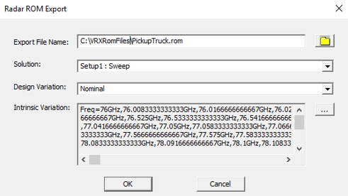
In the Project tree, right-click on the Radiation icon and select Radar ROM Export….

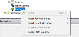
You can then specify the directory and file name for the exported ROM file. Generating the ROM file may take a few minutes while the HFSS post-processor prepares the coherent RCS result data. The exported ROM file is not human readable, but it can be directly imported and used by the ROM-based radar model in VRXPERIENCE Sensors.