


Differences in the contact settings determine how the contacting surfaces separate or slide relative to one another. Definitions of all properties/options under Definition are described in detail in the Contact Region object reference description: Definition. General considerations are discussed here. The following topics are available:
| Defining Type |
| Defining Behavior |
| Using Trim Contact |
| Renaming Contact Regions Based on Geometry Names |
| Saving or Loading Contact Region Settings |
| Resetting Contact Regions to Default Settings |
Type
The contact type specifies how the contact and target surfaces (contact pair) separate or slide relative to each other. Available contact types are listed in the following figure and described briefly here. For further details, see the Contact Region object reference description: Definition.
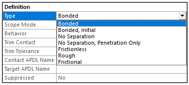
Bonded contact (default) prevents sliding or separating, effectively treating contact regions as if they are glued. Any gaps are closed, and initial penetration is ignored. Since the contact length/area does not change with the application of the load, the solution is linear and computationally efficient.
Autodetected contact regions are defined as bonded by default (Connections > Generate Automatic Connection on Refresh = yes). Bonded contact is ideal when no relative motion is expected, such as welded joints. For modeling separation or stress near interfaces, consider using one of the nonlinear contact types: Frictionless, Rough, Frictional, or No Separation, Penetration Only. These handle gaps and more accurately model the true area of contact, but they may increase solution time and cause convergence issues. If convergence problems arise or if determining the exact area of contact is critical, apply a finer mesh (using Sizing control) on the contact faces or edges. Other contact types are listed below with examples of when they may be useful.
No Separation allows the contact pair to slide without friction but not separate (available only for regions of 3D solid faces or 2D plate edges). The solution is linear. Wipers sliding on a windshield is an example of bodies that slide but do not separate.
Bonded, Initial maintains the initial contact state for the entire analysis. If the contact is initially closed, it remains attached. For an open initial state, the contact remains open even if deformation brings the contact pair close together. Choose Bonded, Initial when the initial contact condition is a key factor in the analysis.
Frictionless models standard unilateral contact: normal pressure equals zero if separation occurs. Both separation and frictionless sliding are allowed. Therefore, gaps can form in the model between contact surfaces depending on the loading. The solution is nonlinear because the area of contact may change as the load is applied. A zero coefficient of friction is assumed. The model should be well constrained when using this contact setting. Weak springs are added to the assembly to help stabilize the model and achieve a reasonable solution. Frictionless contact is applicable when parts can come in and out of contact without any frictional resistance, for example lubricated surfaces.
Rough models frictional contact conditions that prevent sliding, corresponding to an infinite friction coefficient. Separation can occur, and the solution is nonlinear. Only applicable for regions of faces (for 3D solids) or edges (for 2D plates). No automatic closing of gaps is performed. Rough contact is an accurate contact type when parts are expected to stay locked together without any relative motion, for example, a tight interference fit.
No Separation, Penetration Only enforces that surfaces must remain in contact without separating once contact occurs. No gaps are allowed to form between the surfaces once they touch, ensuring that they remain in contact or penetrate each other during the analysis.
This contact type is useful for modeling mechanical systems with components that are expected to remain in contact under load, like press-fit joints or gasketed connections. By preventing separation that may impact the load path or stress distribution, this contact type is particularly advantageous when accurate modeling of the contact pressure distribution is required.
Frictional is the most realistic representation of the contact surfaces. The contact pair can separate and slide with friction (you specify the Friction Coefficient—the frictional resistance value between contact surfaces.). The surfaces in contact can carry shear stresses up to a certain magnitude across their interface before they start sliding relative to each other. The pre-sliding state is called "sticking”. Once an equivalent shear stress is reached, sliding begins as a fraction of the contact pressure.
Forced Frictional Sliding is similar to except that there is no "sticking" state. (Supported only for Rigid Dynamics). A tangent resisting force is applied at each contact point. The tangent force is proportional to the normal contact force.
For the Bonded, , Bonded, Initial, and No Separation, Penetration Only settings, you can simulate the separation of a Contact Region as it reaches some predefined opening criteria using the Contact Debonding feature.
Refer to KEYOPT(12) in the Mechanical APDL Contact Technology Guide for more information about modeling different contact surface behaviors.
Behavior
Specify whether the contact region is modeled as Asymmetric or Symmetric (for 3D face-to-face or 2D edge-to-edge contact). The program automatically sets behavior to Asymmetric for 3D edge-to-edge or face-to-edge contact.
Asymmetric and symmetric contact behavior are described briefly here. Refer to KEYOPT(8) in the Mechanical APDL Contact Technology Guide for more information about asymmetric and symmetric contact selection.
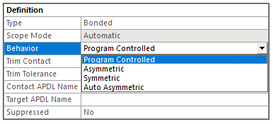
Sets contact pair to one of the following:
Asymmetric behavior designates one surface as the contact side and the other as its counterpart, forming a single contact pair. The nodes on the contact surface are prevented from penetrating the target surface. Asymmetric behavior, also referred to as “one-pass contact,” is usually the most efficient way to model face-to-face contact for solid bodies. Behavior must be set to asymmetric if at least one of the contacting bodies has rigid Stiffness Behavior. Contact results are only available on the contact side for asymmetric behavior.
Auto Asymmetric automatically creates an asymmetric contact pair, when possible, which can boost performance. With this setting, the solver selects the best contact face during the solution phase. [In Explicit Dynamics analyses this option is available for Bonded connections; see Bonded Type.]
Symmetric behavior refers to the designation of each interacting surface as both a contact and a target, resulting in the formation of two distinct contact pairs from the same pair of surfaces. The nodes on the contact and target surface are prevented from interpenetrating. Symmetric contact behavior, also referred to as “two-pass contact”, is less efficient than asymmetric contact. However, many analyses will require its use, typically to reduce penetration, specifically when:
the contact and target sides are not easily distinguished (see Proper designation contact and target sides).
both surfaces have coarse meshes since the symmetric algorithm enforces contact constraint conditions at more surface locations than the asymmetric contact algorithm.
Note that as results are available on both sides of the contact pair, symmetric behavior makes results interpretation tricky. The actual contact result is the average of results from the contact surfaces. The symmetric pairs will have the same contact characteristics (using KEYOPT(8)=1) except when the Nonlinear Adaptive Region object is present.
Program Controlled (Default for the Mechanical APDL solver) behavior depends on the Stiffness Behavior of the bodies in contact, as summarized in the following table.
Body 1 Body 2 Condition Program-controlled behavior flexible flexible Auto asymmetric flexible rigid Asymmetric flexible flexible nonlinear adaptive (NLAD) remeshing is specified Symmetric rigid rigid not applicable, must be defined manually For Rigid-Rigid contact, the behavior property is under-defined for the Program Controlled setting. The validation check is performed at the Contact object level when all environment branches are using the Mechanical APDL solver. If the solver target for one of the environments is other than Mechanical APDL, then this validation check will be carried out at the environment level; the environment branch will become under-defined.
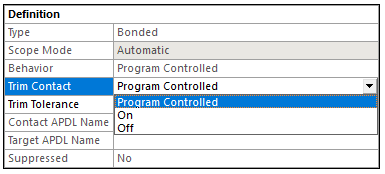
Trim Contact
Trim Contact can speed up solutions by reducing the number of contact elements included. For a Contact Region interface of a Condensed Part, it reduces the number of master DOFs. Elements are included or excluded based on proximity and overlap of a bounding box around each element with a size equal to the Trim Tolerance.
You can choose to turn contact trimming on, off, or have the application control when trimming is performed, Program Controlled, which is the default setting. See Trim Contact for details.
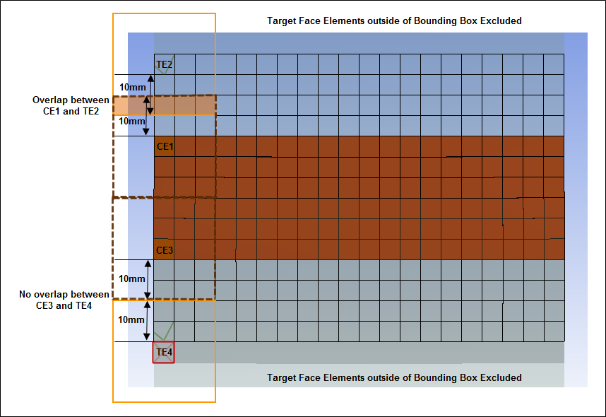
The figure below shows how elements are selected for exclusion using brown contact and blue target elements with an element size of 5 mm. A trim tolerance of 10 mm determines the size of the bounding boxes around both the target and contact elements. If the bounding boxes around the elements overlap, like for CE1 and TE2 shaded orange, TE2 is included in the calculations. If instead there is no overlap, like for CE3 and TE4, which are separated by 20mm, T4 is excluded. Note that the distance between CE3 and TE4 is double the trim tolerance.
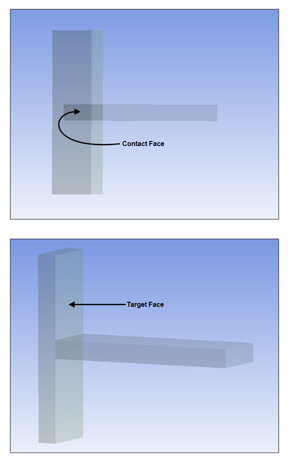
The brown area illustrated below represents the elements from the contact face. On the corresponding target side exist potential elements from the entire target face. The elements of the target face that will be kept are drawn in black. On the target Face, each element bounding box is expanded by 10mm and an overlap is sought against each element from the contact side. Referring to the image below, the bounding boxes between Contact Element 1 (CE1) and Target Element 2 (TE2) overlap and therefore TE2 is included in the analysis. Meanwhile, CE3 and TE4 do not overlap and as a result, TE4 is not included in the analysis. This results in a reduced number of elements in the analysis and, typically, a faster solution.
Renaming Contact Regions Based on Geometry Names
You can change the name of any contact region using the following choices available in the context menu that appears when you click the right mouse button on a particular contact region:
: Enables you to change the contact region name to a name that you type (similar to renaming a file in Windows Explorer).
: Enables you to change the contact region name to include the corresponding names of the items in the Geometry branch of the tree that make up the contact region. The items are separated by the word "To" in the new contact region name. You can change all the contact region names at once by clicking the right mouse button on the Connections branch, then choosing from that context menu. A demonstration of this feature follows.
Refresh the page, as needed, to see the following animation. View online if you are reading the PDF version of the help.
When you change the names of contact regions that involve multiple bodies, the region names change to include the word Multiple instead of the long list of names associated with multiple bodies. An example is Bonded – Multiple To Multiple.
Saving or Loading Contact Region Settings
You can save the configuration settings of a contact region to an XML file. You can also load settings from an XML file to configure other contact regions.
To Save Configuration Settings of a Contact Region:
Select the contact region whose settings you want to save.
Right-click to display the context menu.
Select in the menu. This option does not appear if you selected more than one contact region.
Specify the name and destination of the file. An XML file is created that contains the configuration settings of the contact region.
Note: The XML file contains properties that are universally applied to contact regions. For this reason, source and target geometries are not included in the file.
To Load Configuration Settings to Contact Regions:
Select the contact regions whose settings you want to assign. Use the Shift or Ctrl key for multiple selections.
Right-click to display the context menu.
Select in the menu.
Specify the name and location of the XML file that contains the configuration settings of a contact region. Those settings are applied to the selected contact regions and will appear in the Details view of these regions.
Resetting Contact Regions to Default Settings
You can reset the default configuration settings of selected contact regions.
To Reset Default Configuration Settings of Contact Regions:
Select the contact regions whose settings you want to reset to default values. Use the Shift or Ctrl key for multiple selections.
Right-click to display the context menu.
Select in the menu. Default settings are applied to the selected contact regions and will appear in the Details view of these regions.