


You can generally leave all Contact Region advanced properties set to for most typical simulations. The default program-controlled settings are designed to balance accuracy and computational efficiency for a wide range of contact problems without requiring manual tuning. Leaving advanced contact settings on Program Controlled is a safe and practical choice for many projects. But if you run into problems or want to fine-tune to improve solution stability or speed, the advanced properties are available for you to customize.
Advanced options can be grouped into the following key categories:
| Category | Purpose |
|---|---|
| Formulation Define the core mathematical method and assumptions for solving contact |
|
| Detection & Pinball Control how contact is spatially identified |
|
| Stiffness & Behavior Manage convergence and the physical response of the interface |
|
| Thermal and Electric Behavior Manage flow of quantities across the contact interface for multiphysics simulations |
|
| Rigid Body Motion Handling Handle contact for Rigid Body Dynamics |
|
Definitions of all properties/options under Advanced are described in detail in the Contact Region object reference description: Advanced.
Formulation
While contact Type defines how surfaces interact physically (friction, sliding, separation), contact Formulation defines how the software enforces those interactions mathematically.
Because contacting bodies do not interpenetrate, the application must establish a relationship between the two surfaces to prevent them from passing through each other in the analysis. When the application prevents interpenetration, it is said to enforce "contact compatibility."
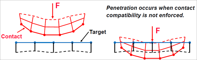
In order to enforce compatibility at the contact interface, the application offers several different contact formulations. These formulations define the solution method used. Formulations fall into three main categories: Penalty-based, Lagrange-based, and specialty.
Penalty-based methods treat contact as a stiff spring that resists penetration. A small, non-physical penetration is allowed, and a contact force is calculated to push the penetrating node back to the target surface. The stiffness of this "spring" determines how much penetration is allowed.
: This is the most basic penalty method. The contact force is directly proportional to the penetration distance and the contact stiffness. While computationally efficient, it can be sensitive to the chosen stiffness value. If the stiffness is too low, excessive penetration occurs, leading to inaccurate results. If it's too high, the solution may struggle to converge. This setting is suited to contact occurring only on an edge or vertex.
Mathematically, the contact force (pressure) calculation is:
or:
The finite contact force,
 , is a function of contact stiffness (or normal stiffness),
  . The higher the contact stiffness, the lower the penetration,
  , as illustrated here.
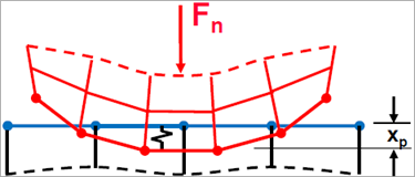
Ideally, for an infinite
 , one would get zero penetration. This is not numerically possible with penalty-based methods, but as long as
  is small or negligible, the solution results are accurate.
: This is the default and most robust penalty-based formulation. It's an enhanced version of the Pure Penalty method that adds a Lagrange multiplier to the force calculation. This extra term helps to reduce the sensitivity to the contact stiffness and provides better control over the penetration. It's known for its good balance of accuracy and computational efficiency, and it often converges more reliably than Pure Penalty.
Mathematically, the main difference between Pure Penalty and Augmented Lagrange methods is that Augmented Lagrange augments the contact force equation:
Because of the extra term
 , the Augmented Lagrange method is less sensitive to the magnitude of the contact stiffness
  .
.


Lagrange-based methods enforce a "no penetration" constraint more strictly by adding an extra degree of freedom (contact pressure) to the model.
: This formulation enforces a nearly zero-penetration condition without requiring a user-defined contact stiffness. It solves for the contact pressure explicitly as a new unknown in the system of equations. While it can be more accurate for problems requiring minimal to zero penetration, it's computationally more expensive and may lead to "chattering," where contact points oscillate between open and closed states, making convergence difficult.
The Normal Lagrange formulation option:
Provides the highest accuracy
Works well with material nonlinearities
Works well with shells or thin layers
Enables interference fit
Allows large sliding
Does not require a normal contact stiffness (zero elastic slip)
Requires that the direct solver be used, which can increase computation requirements
Mathematically, the Normal Lagrange formulation adds an extra degree of freedom (contact pressure) to satisfy contact compatibility. Consequently, instead of resolving contact force as contact stiffness and penetration, contact force (contact pressure) is solved for explicitly as an extra DOF:
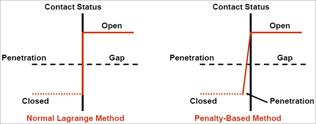
Chattering is an issue that often occurs with the Normal Lagrange method. If no penetration is allowed (left), then the contact status is either open or closed (a step function). This can sometimes make convergence more difficult because contact points may oscillate between an open and closed status—a phenomenon know as "chattering." If some slight penetration is allowed (right), it can make it easier to converge since contact is no longer a step change.
The Normal Lagrange method is highly susceptible to over-constraint. The solver may struggle to satisfy the zero-penetration constraint when other forces and boundary conditions are applied, leading to convergence issues that are a symptom of over-constraint.

Specialty formulation options are available for specific contact scenarios.
(Multi-Point Constraint): This is an excellent, efficient, and accurate method used for and contact Types. It directly ties the degrees of freedom of the contact and target surfaces together using constraint equations, effectively "gluing" them together. Since it's a linear method, it's very fast and can be used for linear and nonlinear analyses including large deformation. This setting is ideal for all linear contact when there is no over-constraint.
The MPC formulation is highly susceptible to over-constraint. This is especially true if you have:
A displacement or other boundary condition applied to the same nodes that are part of the MPC contact region.
Multiple MPC contact regions or other joints that share a common face, edge, or vertex.
MPC contact between rigid bodies or when a rigid body is modeled via a primitive segment.
When you use MPC, you are essentially creating a stiff connection that removes DOFs. If you then apply another constraint that also tries to control those same DOFs (for example, a displacement boundary condition on the same face), you create a redundant and conflicting set of constraints, resulting in an over-constrained system. The solver may issue warnings or errors and may not be able to find a stable solution. In contrast to over-constraining, a properly constrained model has just enough constraints to prevent rigid body motion without being redundant.
: This is a specialized method that is applicable only for contact. It works by "stitching" the contacting surfaces together with massless beam elements, which are computationally efficient for certain applications. This setting is ideal for linear contact when there may be over-constraint.
Contact formulations are summarized in the following table.
| Formulation Option | |||||
|---|---|---|---|---|---|
| Pure Penalty | Augmented Lagrange | Normal Lagrange | MPC | Beam | |
| Convergence | Good convergence behavior (few equilibrium iterations). | Additional equilibrium iterations needed if penetration is too large. | Additional equilibrium iterations needed if chattering is present. | Excellent convergence behavior (one equilibrium iteration). | |
| Contact stiffness | Sensitive to selection of normal contact stiffness. | Less sensitive to selection of normal contact stiffness. | No normal contact stiffness is required. | N/A | |
| Penetration | Contact penetration is present and uncontrolled. | Contact penetration is present but controlled to some degree. | Usually, penetration is near-zero. | No penetration. | Penetration is minimal with a stiff enough material definition. |
| Computational time | Fast | In between Pure Penalty and Normal Lagrange | Slowest | Very fast | Very fast |
| Susceptible to over-constraint[a] | Low, only for high penalty stiffness | Less than Normal Lagrange | High susceptibility | High susceptibility | Low |
| Contact Type | Useful for any type of contact behavior. | Only Bonded & No Separation types. | Bonded only | ||
| Solver | Iterative or direct solvers can be used. | Only direct solver can be used. | Iterative or direct solvers can be used. | ||
| Behavior | Symmetric or Asymmetric contact available. | Asymmetric contact only. | N/A | ||
| Detection | Contact detection at integration points. | Contact detection at nodes. | N/A | ||
[a] Over constraint occurs when a degree of freedom is subjected to multiple, possibly conflicting constraints, such as boundary conditions and MPC constraints, or multiple MPC constraints on the same node.
For additional Mechanical APDL specific information, see KEYOPT(2) in the Mechanical APDL Contact Technology Guide.
Constraint Type
When Formulation = MPC, the Constraint Type property is displayed. It controls how the node DOFs on the contact and target surfaces are "tied" together, either in a rigid or flexible manner, by the MPC equations. It is only available for Bonded and No Separation contact types, which are inherently linear and don't allow for separation.
There are two main options for the Constraint Type property:
Distributed, All Directions: This is the default and most common option. It creates MPC equations that tie the nodes together in all three translational directions (X, Y, and Z). This is like a welded connection, preventing both separation and sliding between the parts. It's suitable for most bonded connections.
Projected, Displacement Only: This option creates MPC equations that tie the nodes together only in the normal direction of the contact surface. It allows for tangential sliding, effectively modeling a No Separation contact with no friction. This option is primarily used for No Separation contact types.
For additional information, see the Controlling Degrees of Freedom Used in the MPC Constraint topic in the Modeling Solid-Solid and Shell-Shell Assemblies section of the Mechanical APDL Contact Technology Guide. Also note that the Mechanical APDL entry for the Constraint Type is KEYOPT(5) for element TARGE170.
Small Sliding
Small Sliding is a contact setting that defines how relative motion between contact and target surfaces is handled during the simulation. Three different sliding behaviors are available: small sliding, finite sliding (also known as large sliding), and adaptive small sliding. The sliding behavior you choose will have an influence on solution robustness, performance, and accuracy. Select the appropriate sliding behavior based on the relative motion of the contact interfaces in your model.
Small Sliding: Assumes relatively-small sliding (less than 20% of the contact length) during the entire analysis. The small sliding logic establishes the contact node-to-target element relationship at the very beginning of the analysis and maintains it throughout. This means a contact node will always interact with the same target element, even if the body it's on rotates or moves. Small sliding is faster and more stable, because it avoids having to constantly search for a new contact location.
Finite Sliding: Allows for arbitrary separation, sliding, and rotation of the contact interfaces. In general, each contact detection point can interact with different target elements, depending on the contact status (open, closed, or sliding). The program re-forms nodal connectivity of the contact element based on the current configuration at each equilibrium iteration. The finite-sliding logic is computationally expensive, but guarantees solution accuracy.
Set Finite Sliding when contact surfaces are expected to slide significantly across one another, you have rotational or translational motion between contact bodies, or you're doing a nonlinear or large deformation analysis.
Adaptive Small Sliding: A smart, in-between option designed to give you the speed of Small Sliding with the flexibility of Finite Sliding, but only if needed. It's a dynamic algorithm that starts with the small sliding assumption for efficiency but is designed to detect when the sliding is becoming too large. When this happens, it can "adapt" and re-establish the contact connectivity at the beginning of a new substep, which helps to maintain accuracy and prevent non-physical results without the constant re-calculation of the full finite sliding method.
The Program Controlled setting automatically sets the Small Sliding to On in most situations if Large Deflection = Off or Type = contact. You can change the default behavior: File > > Mechanical:Connections > Small Sliding.
Small Sliding options are summarized in the following table.
| Small Sliding | Finite Sliding | Adaptive Small Sliding | |
|---|---|---|---|
| Assumption/Description | Assumes minimal relative motion | Allows full (large) sliding and contact searching | Starts as small, switches to finite if needed |
| Speed | Fast | Slower | Fast (initially) |
| Flexibility | Low | High | Smart |
| Use Case | Static or tight fits, small motion, small vibrations, thermal expansion | Mechanisms, large motion, bearings, gears, cams, sliders | Mixed or uncertain motion scenarios |
For additional information, see the Selecting a Sliding Behavior topic in the Mechanical APDL Contact Technology Guide.
Detection Method
Detection Method determines where on the contact and target surfaces the software looks for, and calculates, contact interactions. It defines the "contact points" that are used to enforce the no-penetration condition between parts. This is an important setting because it directly influences the accuracy and stability of your contact simulation. It is applicable to 3D face-to-face and 2D edge-to-edge contact.
The default setting is Program Controlled, which automatically selects a method based on the contact formulation and other factors. For example, it often defaults to a method based on Gauss integration points for Augmented Lagrange and Pure Penalty formulations and a nodal-based method for MPC or Normal Lagrange.
You typically only need to change the detection method from its default setting when you're facing specific convergence issues or if you need to improve the accuracy of a particular result. Here are some scenarios where you would consider changing the setting:
Convergence Problems: If your simulation is failing to converge, especially at the beginning of a load step, changing the detection method can sometimes help. For instance, Nodal-Projected Normal From Contact is often more robust and can improve convergence for many nonlinear contact problems.
Contact on Edges and Corners: For problems involving contact at sharp corners or edges, nodal-based methods like Nodal - Normal to Target or Nodal - Normal From Contact are often recommended.
Curved or Coarse Meshes: The Nodal-Projected Normal From Contact method is particularly useful for models with curved surfaces or meshes that are not fine enough at the contact interface. It provides a more accurate distribution of contact forces in these situations.
Specialized Applications: Specific types of analyses, like those involving gasket layers or acoustic-structure interaction (ASI), have specialized recommendations for contact detection, often favoring the projected normal method.
Interference Fits: When modeling interference or press-fit problems, changing the detection method can help achieve better results and improve convergence.
For additional Mechanical APDL information, see Selecting Location of Contact Detection (specifically, KEYOPT(4) information) in the Mechanical APDL Contact Technology Guide.
Penetration Tolerance
Penetration Tolerance is a convergence criterion for contact analysis. It specifies the maximum allowable physical overlap (penetration) between two contacting bodies for the solution to be considered converged.
When running a nonlinear contact analysis, the solver iterates to find a balanced state where forces and displacements are in equilibrium. With penalty-based formulations, a small amount of penetration is necessary to generate the contact force that prevents further overlap. The solver calculates this penetration and compares it to the specified tolerance. If the penetration is within this tolerance, the contact is considered to be "in contact" and the solver can move on. If the penetration exceeds this value, the solution is considered unconverged (the model is still deforming significantly at the contact interface and has not reached a stable state) even if other convergence criteria (like force and displacement residuals) are met.
The default value for Penetration Tolerance is 10% of the underlying element size. This is a program-controlled value that is automatically calculated based on the mesh density in the contact region. You can change the Penetration Tolerance from its default by specifying either a factor (Penetration Tolerance Factor)—for example, a factor of 0.05 would set the tolerance to 5% of the element size, or an absolute value (Penetration Tolerance Value) in length units.
Decreasing the tolerance (for example, to a factor of 0.01) makes the analysis more stringent, requiring less penetration for convergence. This can lead to more accurate results, especially for high-precision analyses, but may also make it more difficult for the solution to converge.
Increasing the tolerance allows for more overlap, which can help with convergence issues but may sacrifice accuracy if the penetration is excessive relative to the overall deformation or part size. You should ensure that the contact penetration is “small” relative to the local displacements.
Note: When viewing the Connections Worksheet, a displays as a negative number and a displays as a positive number.
For additional information, see the Determining Contact Stiffness and Allowable Penetration, specifically Using FKN and FTOLN, section of the Mechanical APDL Contact Technology Guide (Surface-to-Surface Contact).
Elastic Slip Tolerance
Elastic Slip Tolerance specifies the maximum allowable "elastic slip" in the tangential direction for frictional contact. When two surfaces are in a sticking state (that is, pre-sliding but not sliding), a small amount of deformation can still occur at the contact interface due to tangential forces. This micro-movement is called elastic slip. It's the tangential equivalent of the small penetration that occurs in the normal direction. The application uses a tangential stiffness to resist this slip, similar to how normal stiffness resists penetration.
The default value for Elastic Slip Tolerance is 1% of the average contact element length. This provides a good balance between accuracy and convergence for most problems. You can change the Elastic Slip Tolerance from its default by specifying either a factor (Elastic Slip Tolerance Factor) or an absolute value (Elastic Slip Tolerance Value) in length units.
The Program Controlled (default) setting works for most cases, but you may want to manually adjust the tolerance in these scenarios:
To resolve convergence issues: If your frictional contact analysis fails to converge and you suspect it's due to the contact surfaces "bouncing" between sticking and sliding states (chattering), increasing the elastic slip tolerance can help stabilize the solution.
To increase accuracy: In high-precision analyses where the onset of sliding is critical, you might need to decrease the tolerance to ensure the model accurately captures the sticking behavior. Decreasing the tolerance forces the solver to be more stringent, requiring less elastic slip. This can lead to a more accurate solution but may cause chattering or convergence difficulties if the tangential forces are large or if the model is on the cusp of sliding.
Applicable when the Formulation = or when the contact stiffness is set to update each iteration (Update Stiffness = or ). Not applicable when the contact Type = or .
Note: When viewing the Connections Worksheet, a displays as a negative number and a displays as a positive number.
For additional information, see the Determining Contact Stiffness and Allowable Penetration, specifically Using FKT and SLTO, section of the Mechanical APDL Contact Technology Guide (Surface-to-Surface Contact).
Normal Stiffness
For penalty-based formulations, the Normal Stiffness, , is the stiffness of an imaginary stiff spring placed between the contact surfaces. It provides a “restoring force” to enable penetrating nodes to stay within the defined penetration tolerance and is a key factor in controlling the balance between solution accuracy and convergence. A higher value reduces penetration but can cause convergence issues, while
a lower value allows more penetration but is generally more stable.
By default, the application calculates a reasonable value automatically, usually based on the stiffness of the underlying elements. You can, however, override this by setting a Factor (define a Normal Stiffness Factor) or an Absolute Value (define a Normal Stiffness Value).
Higher Normal Stiffness: A high value for Normal Stiffness results in a larger restorative force for a given amount of penetration. This leads to less penetration and more accurate results, which is generally desirable. However, an excessively high stiffness can make the solver "chatter" between contact states and cause significant convergence difficulties, leading to a non-converged solution.
Lower Normal Stiffness: A lower value results in less force to resist penetration. This can help improve convergence by making the system more flexible, but it can also lead to an unrealistic amount of penetration, compromising the accuracy of your results, especially for problems where contact stress and penetration are critical to the solution (for example, press-fits).
The goal is to find a balance: a stiffness high enough to keep penetration acceptably low without hindering convergence. The default value is appropriate for bulk deformation. If bending deformation dominates, use a smaller factor (0.01 - 0.1). For most problems, the program-controlled default works well, but for models with complex
contact or convergence issues, adjusting this value is a common troubleshooting step.
For additional information specific to Mechanical APDL, see the following sections:
Determining Contact Stiffness and Allowable Penetration section of the Mechanical APDL Contact Technology Guide (Surface-to-Surface Contact).
Using FKN and FTOLN section of the Mechanical APDL Contact Technology Guide (Surface-to-Surface Contact).
Update Stiffness
This property enables you to specify if the program should update (change) the contact stiffness during the solution. If you choose any of these stiffness update settings, the application modifies the stiffness (raises/lowers/leaves unchanged) based on the physics of the model (that is, the underlying element stress and penetration). To use the options of this property, you need to set the Formulation property to either or , the two formulations where contact stiffness is applicable. For the option, the Formulation property must be set to .
An advantage of specifying an Update Stiffness setting is that stiffness is automatically determined that allows both convergence and minimal penetration. Also, if this setting is used, problems may converge in a Newton-Raphson sense, that would not otherwise.
You can use a Result Tracker to monitor a changing contact stiffness throughout the solution. Property options include:
| Option | Description |
|---|---|
| Program Controlled (default) | The application sets the property to for contacts between two rigid bodies and to for all other cases. You can change the default using the Options dialog. |
| Never | Turn off Update Stiffness feature. |
| Update stiffness at the end of each equilibrium iteration. This choice is recommended if you are unsure of a . | |
| Updates stiffness at the end of each equilibrium iteration by more aggressively changing the value range. | |
| This setting requires you to first set the Type property to either or and the Formulation property to . When selected, the Pressure at Zero Penetration and the Initial Clearance properties display. This option updates stiffness using an exponential pressure-penetration relationship. For detailed information about this option, see the Exponential Pressure-Penetration Relationship (KEYOPT(6) = 3) topic (of the Set the Real Constants and Element KEYOPTS section) in the Mechanical APDL Contact Technology Guide. |
Electric Capacitance
You can specify the electric contact capacitance value used in an electric contact simulation.
Pressure at Zero Penetration and Initial Clearance
Using a uniform normal contact stiffness for each contact pair may cause convergence problems. The exponential pressure-penetration relationship (KEYOPT(6) = 3 in Mechanical APDL) based on default values for zero penetration pressure and initial clearance (PZER and CZER in Mechanical APDL), results in non-uniform contact stiffness. This law smooths contact behavior in cases like self-contact, soft materials, large initial gaps, uneven meshes, and interface chattering.
Pressure at Zero Penetration defines the pressure when there is zero penetration between contact and target geometries, and Initial clearance specifies the initial clearance or gap at which the contact pressure begins to act on the contact and target geometries. The table below lists the options for both of these values.
For a more detailed description of the exponential pressure-penetration law, see the Exponential Pressure-Penetration Relationship (KEYOPT(6) = 3) topic (of the Set the Real Constants and Element KEYOPTS section) in the Mechanical APDL Contact Technology Guide for more details.
| Option | Description | Mechanical APDL Reference |
|---|---|---|
| (default) | The application automatically calculates and selects default pressure values. | KEYOPT(6) = 3 |
| Using this option, you can manually specify a pressure value (units of pressure) or an initial clearance (length units). Only non-zero positive values are valid. | ||
| Manually specify a factor of the default pressure (or clearance) value or (0 ≥ factor < 1.0). This entry is unitless. |
Stabilization Damping Factor
A defined contact may initially have a near open status due to small gaps, which can cause rigid body motion. The Stabilization Damping Factor adds a small, artificial damping force between the contacting surfaces to damp the relative motion and prevent rigid body motion until contact is properly established. This contact damping factor is applied in the contact normal direction, and it is valid only for the , , and contact types.
Damping is applied during each load step with open contact status, and the stabilization damping factor should be set high enough to prevent rigid body motion without compromising solution convergence.
The default value in the Mechanical application (0) does not activate
damping. For non-zero entries, damping is always activated regardless of the contact
status of the previous substeps, and the solver uses KEYOPT(15) = 3 to apply stabilization
damping. Ansys recommends a range of 0.1 (low damping) to
10 (high damping).
For more information, see Real Constant FDMN.
Thermal Conductance
Controls the thermal contact conductance value used in a thermal contact simulation. Use realistic values for thermal simulations involving heat conduction through contact. Change it if contact pressure, roughness, or material properties influence thermal behavior.
Pinball Region
The Pinball Region is a sphere with a defined radius centered around the nodes of the contact body. The solver performs detailed contact calculations only for nodes on the target body that are within the pinball region (“near-field”). If the pinball region is too small, the solver might miss actual contact points, especially if there is an initial gap between contact surfaces. If it is too large, the solver performs unnecessary calculations for nodes that are not actually in contact, increasing solution time and memory usage. The Program Controlled (default) setting works for most cases, but you may want to manually adjust the pinball radius in these scenarios:
To account for initial gaps/penetration: If your model has intentional initial gaps or penetration between contact and target surfaces, a larger pinball radius may be required.
To address convergence issues: If your solution is not converging, a smaller pinball radius can sometimes help.
Note that for the and contact types, use caution when specifying a large pinball region, as any area within them is treated as in contact. For other contact types, this is less critical since the application performs additional calculations to determine true contact between bodies. Also, large gaps may transmit artificial moments at boundaries.
- Rigid Dynamics Solver
For the Rigid Dynamics solver, the Pinball Region property is used to control the touching tolerance. By default, the Rigid Dynamics solver automatically computes the touching tolerance using the sizes of the surfaces in the contact region. These default values are sufficient in most of cases, but inadequate touching tolerance may arise in cases where contact surfaces are especially large or small (small fillet for instance).
Electric Conductance
Controls the electric contact conductance value used in an electric contact simulation.
With the Program Controlled setting, the application calculates an electric contact conductance value that is high enough to simulate near-perfect contact and minimal resistance, based on electric conductivities and model size. To specify a value, choose Manual and enter a value in units of electric conductance per area.
Note: The Electric Analysis result, Joule Heat, when generated by nonzero contact resistance, is not supported.
Time Step Controls
Allows you to specify if changes in contact behavior should control automatic time stepping. This choice is displayed only for nonlinear contact (Type is set to , Frictionless, Rough, or Frictional). Options are:
| Option | Description |
|---|---|
| None (default) | Contact behavior does not control automatic time stepping. This option is appropriate for most analyses when automatic time stepping is activated and a small time step size is allowed. |
| Automatic Bisection | Contact behavior is reviewed at the end of each substep to determine whether excessive penetration or drastic changes in contact status have occurred. If so, the substep is reevaluated using a time increment that is bisected (reduced by half). |
| Predict for Impact | Performs same bisection on the basis of contact as the Automatic Bisection option and also predicts the minimal time increment needed to detect changes in contact behavior. This option is recommended if you anticipate impact in the analysis. |
| Use Impact Constraints | Activates impact constraints with automatic adjustment of the time increment. This option includes constraints on penetration and relative velocity to more accurately predict the duration of impact and the rebound velocities after separation. |
Restitution Factor—Rigid Dynamics Solver Only
In a rigid dynamics analysis, the Restitution Factor (under Advanced) represents the energy loss during shock. It is the ratio of relative velocity before and after impact, ranging from 0 to 1. The default value of 1 means no energy loss or a perfectly elastic collision.
Continuous Distance Computation—Rigid Dynamics Solver Only
Continuous Distance Computation is applicable only for a rigid dynamics analysis. By default, it is disabled by the Program Controlled setting, and the distance is calculated only when the contact bodies are significantly close in contact. Select Yes to force distance computation, even when contact bodies are distant. See for further information).