


VM-LSDYNA-SOLVE-056
VM-LSDYNA-SOLVE-056
Transient Response of a Two-Mass-Spring System
Overview
| Reference: | Vierck, R.K. (1979). Vibration Analysis (2nd Edition). Harper & Row, Section 5-8. |
| Analysis Type(s): | Explicit Dynamics Analysis |
| Element Type(s): | 1D Discrete Elements, Mass Elements |
| Input Files: | Link to Input Files Download Page |
Test Case
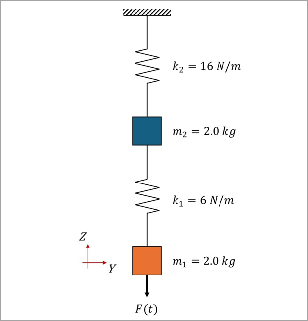
This test case models a system composed of two masses and two springs, illustrated in Figure 188. Both masses are 2 kg, the stiffness of spring 1 is 6 N/m, and the stiffness of spring 2 is 16 N/m. Mass 1 is subjected to a pulse load F(t) with amplitude F0 of 50 N and duration td of 1.8 s. The objective is to validate the displacement profile of each mass. The spring length is arbitrarily defined as 1.0 m.
This problem is also presented in test case VM182 in the Mechanical APDL Verification Manual.
Figure 188: Schematic of the test case, including domain geometry, main dimensions, and boundary conditions
The following table lists the main parameters of the test case, which follow the International System of Units (length in m, time in s, mass in kg, force in N, and pressure in Pa).
| Material Properties | Geometric Properties | Loading |
|---|---|---|
|
Concentrated masses m1, m2 = 2 kg Stiffness constant of spring 1 k1 = 6 N/m Stiffness constant of spring 2 k2 = 16 N/m |
Spring length l = 1.0 m |
Pulse load F(t) with amplitude F0 of 50 N and duration td of 1.8 s |
Analysis Assumptions and Modeling Notes
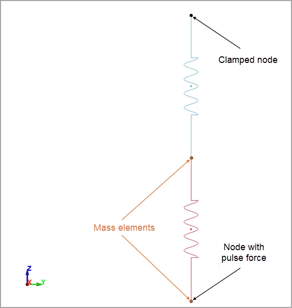
Figure 189: Model setup in LS-DYNA application of the 1D dynamics analysis of a two-mass-spring system
The variables  ,
,  ,
,  , and
, and  can be used to simplify the general solution of the system:
 | (38) |
Where  and
and  are the concentrated masses, and
  and
and  are the spring constants of springs 1 and 2. The natural frequency and
amplitude ratio of the two modes of the system can then be calculated:
are the spring constants of springs 1 and 2. The natural frequency and
amplitude ratio of the two modes of the system can then be calculated:
 | (39) |
 | (40) |
Where  and
and  are the natural frequencies and amplitude ratios of the system for modes 1
and 2, respectively. During the pulse load (
are the natural frequencies and amplitude ratios of the system for modes 1
and 2, respectively. During the pulse load ( ), the motion of the two masses is calculated as:
 | (41) |
 | (42) |
Where  and
and  are the displacements of masses 1 and 2, and
  is the amplitude of each vibration mode of mass 1. After the pulse load (
 ), the motion of the two masses becomes:
 | (43) |
 | (44) |
Two parts are defined to represent the two springs, being meshed with 1D discrete elements. The springs use elastic spring material cards (*MAT_SPRING_ELASTIC) with their respective stiffness constants. Two mass elements of 2.0 kg are defined using *ELEMENT_MASS for the middle and bottom nodes. The top node, connected to spring 2, has its translational and rotational constraints defined with *BOUNDARY_SPC_NODE. A pulse load is prescribed to the bottom node, connected to spring 1, using *LOAD_NODE_POINT. A termination time of 2.40 s is defined using *CONTROL_TERMINATION.
Results Comparison
The displacement profile of each mass is shown in Figure 190.
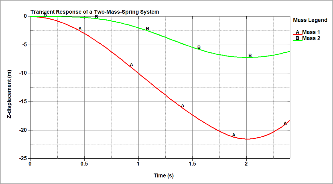
To quantify the error between the theoretical and LS-DYNA results, the mass displacements at 1.3 s and 2.4 s are calculated with their relative errors and shown in the following table. This comparison verifies the agreement between the displacements.
| Results | Target | LS-DYNA Solver | Error (%) |
|---|---|---|---|
| Displacement of mass 1 (m) at 1.3 s | -14.477 | -14.504 | 0.19% |
| Displacement of mass 2 (m) at 1.3 s | -3.987 | -4.001 | 0.34% |
| Displacement of mass 1 (m) at 2.4 s | -18.322 | -18.353 | 0.17% |
| Displacement of mass 2 (m) at 2.4 s | -6.137 | -6.138 | 0.03% |