


VM-LSDYNA-SOLVE-053
VM-LSDYNA-SOLVE-053
Seismic Response of a Mass-Spring System
Overview
| Reference: | Thomson, W.T. (1971). Vibration Theory and Applications (3rd impression). Prentice-Hall, Inc., p. 78, example 3.11-1. |
| Analysis Type(s): | Implicit Modal, Harmonic Analysis |
| Element Type(s): | 1D Discrete Element, Mass Element |
| Input Files: | Link to Input Files Download Page |
Test Case
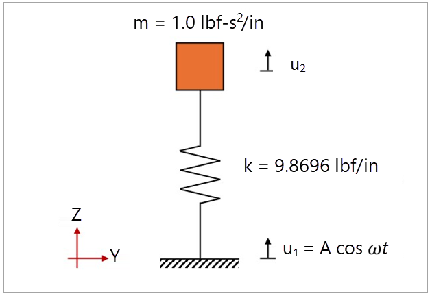
This test case models a vibrometer, consisting of a mass-spring system with base
excitation. The mass is 1.0 lbf-s2/in, and the
spring stiffness is 9.8696 lbf/in. The base oscillates with an amplitude of 1
in and frequency of 22.43537 rad/s. The objective is to validate the natural
frequency of the system  and the relative motion of the vibrometer. The spring length is arbitrarily
defined as 5.0 in. The image below illustrates the domain dimensions and
boundary conditions.
and the relative motion of the vibrometer. The spring length is arbitrarily
defined as 5.0 in. The image below illustrates the domain dimensions and
boundary conditions.
This problem is also presented in test case VM69 in the Mechanical APDL Verification Manual.
The following table lists the main parameters of the test case, which uses the following system of units: length in in, time in s, mass in lbf-s2/in, force in lbf, and pressure in psi.
| Material Properties | Geometric Properties | Loading |
|---|---|---|
|
Stiffness constant of spring
Seismic mass m = 1.0 lbf-s2/in |
Spring length
|
Base oscillation ( |


Analysis Assumptions and Modeling Notes
The natural frequency of a mass-spring system can be calculated as:
 | (28) |
where
 is the stiffness constant of the spring is the stiffness constant of the spring |
and  is the concentrated mass is the concentrated mass |
For the current test case, the natural frequency of the system is 0.5 Hz.
The relative displacement between the seismic mass and the frame,  , can be calculated as:
 | (29) |
where
 is the base motion frequency is the base motion frequency |
 is the natural frequency of the system is the natural frequency of the system |
and  is the amplitude of the base oscillation is the amplitude of the base oscillation |
For the current test case, the relative motion is
1.02 in.
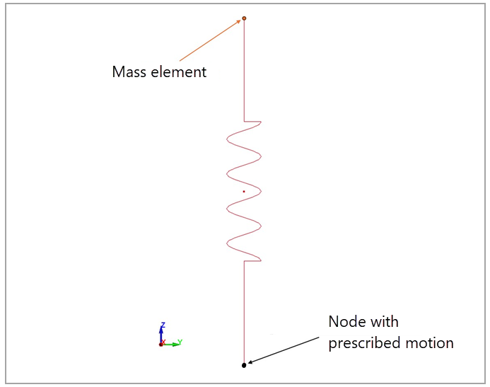
One part is defined to represent the spring, being meshed with a 1D discrete element. This element has a length of 5 in and uses an elastic spring material card (*MAT_SPRING_ELASTIC) with stiffness of 9.8696 lbf/in. A mass element of 1.0 lbf-s2/in is defined for the top node of the structure using *ELEMENT_MASS. Both nodes have their motion restricted to z-translation only using *BOUNDARY_SPC_NODE. The keywords *CONTROL_IMPLICIT_GENERAL (IMFLAG=1) and *CONTROL_IMPLICIT_EIGENVALUE (NEIG=1) are used to activate the implicit eigenvalue analysis with one eigenvalue to be extracted.
The keywords *FREQUENCY_DOMAIN_SSD, *DATABASE_FREQUENCY_ASCII_NODOUT_SSD, and *DATABASE_FREQUENCY_BINARY_D3SSD are used to activate and create the ASCII and binary output files for the steady-state dynamic analysis generated due to the harmonic excitation of the base.
Results Comparison
The visualization of the fundamental mode can be performed by reading the d3eigv file, generated for the modal analysis. The relative displacement of the nodes can be observed in the nodout_ssd and d3ssd files, generated for the harmonic analysis. To quantify the error between the theoretical and LS-DYNA results, the natural frequency of the mass-spring system, the relative displacement between the ends, and their relative errors are calculated and shown in the following table. This comparison verifies the agreement between the natural frequencies and relative displacements.
| Results | Target | LS-DYNA Solver | Error (%) |
|---|---|---|---|
Natural Frequency  (Hz) (Hz) | 0.5000 | 0.5000 | 0.00 |
Relative Displacement  (in) (in) | 1.0200 | 1.0200 | 0.00 |