


VM-LSDYNA-SOLVE-047
VM-LSDYNA-SOLVE-047
Axial Natural Frequency of Hat Beams
Overview
| Reference: | Blevins, R. J. (1979). Formula for Natural Frequency and Mode Shape. Van Nostrand Reinhold Company Inc. |
| Analysis Type(s): | Implicit Vibration Analysis |
| Element Type(s): | 3D Hexahedral |
| Input Files: | Link to Input Files Download Page |
Test Case Description
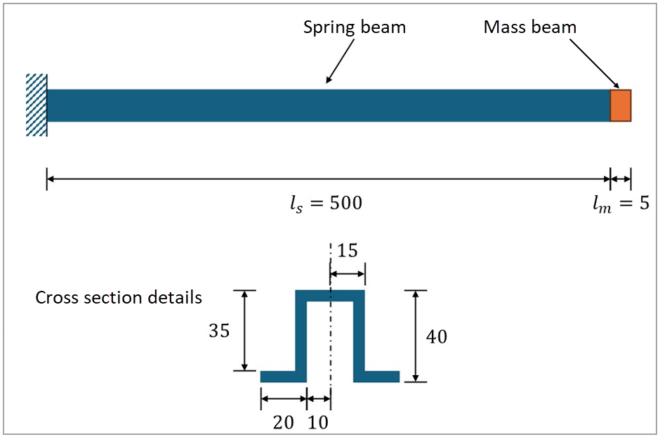
This test case simulates the vibration of a spring-mass system composed of two collinear hat bars. The objective is to validate the axial natural frequency of the structure. The mass beam (shorter bar) has a length of 5 mm. The spring beam (longer bar) has a length of 500 mm. The spring beam is clamped at one end and connected to the mass beam at the other end.
Figure 166 shows a schematic of the test case, including domain geometry, main dimensions, and boundary conditions (all dimensions in mm).
The following table lists the main parameters of the test case. The test case uses the following system of units: length in mm, time in ms, mass in kg, force in kN, and pressure in GPa.
| Material Properties | Geometric Properties |
|---|---|
| Spring Beam Young's modulus (E) = 110 GPa Poisson's ratio (ν) = 0.34 Density (ρ) = 1·10-17 kg/mm3 Mass BeamYoung’s modulus (E) = 200 GPa Poisson’s ratio (ν) = 0 Density (ρ) = 7.85·10-4 kg/mm3 |
Spring beam length (ls) = 500 mm Mass beam length (lm) = 5 mm |
For a uniform, linear elastic, clamped spring with a concentrated mass, the approximate formula to calculate the axial natural frequency  is given as:
 | (18) |
where
 is the stiffness constant is the stiffness constant |
 is the concentrated mass is the concentrated mass |
 is the mass of the spring is the mass of the spring |
In the current scenario, the spring beam acts as the clamped spring and the mass beam as the concentrated mass. For the spring beam, the stiffness constant can be calculated as:
 | (19) |
Where:
 is Young's modulus of the spring beam. is Young's modulus of the spring beam. |
 is the cross-sectional area of the spring beam. is the cross-sectional area of the spring beam. |
 is the length of the spring beam. is the length of the spring beam. |
The axial natural frequency of the spring-mass system formed of two hat beams can be obtained by substituting the above equations:
 | (20) |
Where:
 is the mass of the mass beam is the mass of the mass beam |
 is the mass of the spring beam is the mass of the spring beam |
For the current test case, the mass of the mass beam is 2.551 kg, and the mass of the spring beam is 3.25 10-12 kg. Therefore, the axial natural frequency is 1.19155 kHz.
Analysis Assumptions and Modeling Notes
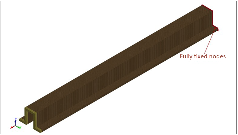
Two parts are defined to represent the mass beam (ID 1) and the spring beam (ID 2). Both are meshed with 3D hexahedral elements of 1 mm length, using the constant-stress solid formulation (*SECTION_SOLID, ELFORM=1) and an elastic material model (*MAT_ELASTIC) with properties listed in the Material Properties table. The nodes on the end surface of the spring beam are grouped with *SET_NODE_LIST, and *BOUNDARY_SPC_SET applies full translational and rotational constraints about all three axes to this node set. The keywords *CONTROL_IMPLICIT_GENERAL (IMFLAG=1), *CONTROL_IMPLICIT_DYNAMICS (IMASS=0), and *CONTROL_IMPLICIT_EIGENVALUE (NEIG=6) are used to activate the implicit eigenvalue, static analysis with six eigenvalues to be extracted.
Results Comparison
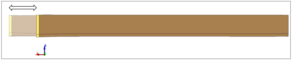
The configuration of the hat beams for the axial mode is shown below. The visualization of the axial (sixth) mode is performed by reading the d3eigv file, generated for the modal analysis.
To quantify the error between the theoretical and LS-DYNA results, the axial natural frequency of the hat beams and its relative error is calculated and shown in the following table. This comparison verifies the excellent agreement between the fundamental frequencies.
Table 18: Comparison between the fundamental frequency of the hat beams calculated using the modal theory and the LS-DYNA model
| Results | Target | LS-DYNA Solver | Error (%) |
|---|---|---|---|
| Axial Natural Frequency (kHz) | 1.19155 | 1.19176 | 0.02% |