


VM-LSDYNA-IMPACT-003
VM-LSDYNA-IMPACT-003
Tensile Elastic Wave Analysis in a 2D Split-Hopinson Pressure Bar
Overview
| Reference: |
Shin, H., Kim, S., & Kim, J.-B. (2020). Stress transfer mechanism of flange in split Hopkinson tension bar. Applied Sciences, 10(19), 7601. https://doi.org/10.3390/app10217601 Shin, H., & Kim, D. (2020). One dimensional analyses of striker impact on bar with different general impedance. Proceedings of the Institution of Mechanical Engineers, Part C: Journal of Mechanical Engineering Science, 234(3), 589–608. https://doi.org/10.1177/0954406219877210 Meyers, M. A. (1994). Dynamic behavior of materials. John Wiley & Sons. |
| Analysis Type(s): | Explicit Impact Dynamics |
| Element Type(s): | 2D Shell Mesh with Quadrilateral Elements |
| Input Files: | Link to Input Files Download Page |
Test Case
The finite element simulation presented in this test case models the two-dimensional (2D) impact of a hollow cylinder (striker) on a flange connected to a long bar (incident bar). The test case is a 2D axisymmetric adaptation of VM-LSDYNA-IMPACT-002, Tensile Elastic Wave Analysis in a 3D Split-Hopkinson Pressure Bar.
The simulation results show the magnitude and duration of the first tensile stress wave transmitted to the bar after impact. These values are validated against calculated values for an identical impact scenario to verify the accuracy of the LS-DYNA explicit solver.
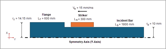
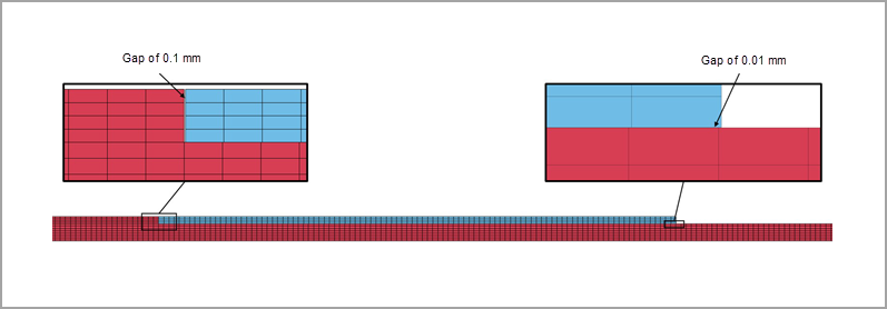
Figure 361 provides a schematic of the test case. The incident bar is modeled as an L-shape to represent a two-dimensional stepped cylinder, and the striker is modeled as a rectangular shell representing a two-dimensional hollow cylinder positioned around the incident bar. The striker rests 0.1 mm from the flange and 0.01 mm from the outer surface of the incident bar. The striker has an initial velocity, Vs, of 15 mm/ms toward the flange.
The table that follows shows the corresponding material and geometric properties as well as the loading conditions. The material of both parts is linear elastic and isotropic with typical steel properties.
| Material Properties | Geometric Properties | Loading |
|---|---|---|
|
Young's modulus (E) = 210 GPa Poisson's ratio (ν) = 0.3 Density (ρ) = 7.8 · 10-6 kg/mm3 |
Bar diameter (Db) = 20 mm Flange height (Hf) = 4.15 mm Bar length (Lb) = 1800 mm Flange length (Lf) = 600 mm Striker length (Ls) = 300 mm | Initial velocity (Vs) = 15 mm/ms |
This test case uses length in mm, time in ms, mass in kg, force in kN, and stress in GPa.
Analysis Assumptions
In the tensile configuration of a Split-Hopkinson Pressure Bar, a tensile stress wave is generated and propagates through the incident bar. This wave is transmitted to the rest of the testing apparatus, which includes the specimen and the transmission bar attached to the incident bar’s end. However, in the current test case, only the tensile stress wave within the incident bar is considered. The specimen and transmission bar are excluded from the analysis.
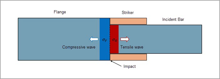
The striker impacts the flanged section of the incident bar, generating two primary stress waves: a compressive stress wave through the flange (moving right to left) and a tensile stress wave through the incident bar (moving left to right).
Figure 362 illustrates the propagation of this tensile stress wave moments after impact.
When waves reach the end of a given structure, they reflect back in the opposite direction. After the striker impacts the flange, the total length of the resulting compressive wave traveling through the striker and reflecting back is then twice the length of the striker ( ). Therefore, if the length of the flange (
 ) is shorter than that of the striker (
 ), the first wave reflected back through the flange would combine with the first tensile stress wave in the incident bar. In the current test case, the length of the flange is twice that of the striker (
 ), so the waves do not combine.
The duration period of the first stress wave at a fixed particle in the incident bar ( ) can be calculated using the striker’s length (
 ) and the speed of sound in the material (
 ):
):
 | (119) |
The speed of sound in the material ( ) can be calculated using its Young’s modulus (
 ) and density (
 ). Material properties for the current test case are included in the test case description.
 | (120) |
The resulting speed of sound for the steel-like material used in this test case is 5,189 mm/ms. Therefore, using Equation 119, the duration period ( ) of the first stress wave in the incident bar is 0.1156 ms.
To calculate the magnitude of the first bar wave ( ), Equation 121 is used to obtain the force equilibrium at the impact plane.
 | (121) |
Where:
 represents the axial stress of the striker ( represents the axial stress of the striker ( ), flange ( ), flange ( ), and incident bar ( ), and incident bar ( ). ). |
 represents the cross-sectional area of the striker ( represents the cross-sectional area of the striker ( ), flange ( ), flange ( ), and incident bar ( ), and incident bar ( ). ). |
Using momentum conservation, the axial stress of each component ( ,
,  ,
,  ) caused by an impact can be calculated using Equation 122:
 | (122) |
Where:
 is the change of velocity in the structure's particles. is the change of velocity in the structure's particles. |
Immediately after the impact, the particle velocity at the impact plane,  , is the same for the three structures. Since the rest of the striker is moving with a velocity of
  , its velocity change is
  . Substituting Equation 122 in Equation 121:
 | (123) |
The acoustic impedance of a structure (  ) is calculated as the product of its cross-sectional area (
  ), its density (
  ), and the speed of sound in the material (
  ). Therefore, the particle velocity can be obtained:
 | (124) |
 | (125) |
The magnitude of the tensile stress in the incident bar can then be calculated by substituting equation Equation 125 in Equation 121:
 | (126) |
Therefore, the magnitude of the first stress wave transmitted to the incident bar is 0.1518 GPa.
Modeling Notes
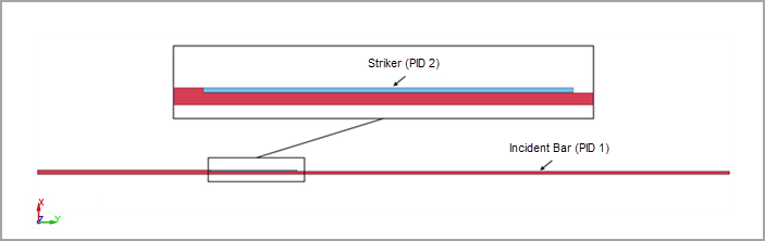
In the simulation, two parts are defined: one to represent the incident bar with flange (PID 1) and another to represent the striker (PID 2). These parts are meshed with 2D quadrilateral shell elements with a length of 3 mm in the axial direction and lengths from 1.0375 mm to 1.25 mm in the radial direction. The parts use a the axisymmetric shell element formulation (*SECTION_SOLID with ELFORM=15), which considers the y-axis the axis of symmetry (see Figure 361).
The parts use an elastic material card (*MAT_ELASTIC) with density of 7.8⋅10-6 kg/mm3, Young’s modulus of 210 GPa, and Poisson’s ratio of 0.3.
The contact definition between the striker and the flange is defined with the keyword *CONTACT_2D_AUTOMATIC_SURFACE_TO_SURFACE using the sets of nodes that represent the contact surfaces.
The initial velocity of the striker is defined using the keyword *INITIAL_VELOCITY_GENERATION with a translational velocity in global y-direction of -15 mm/ms.
The keyword *CONTROL_TERMINATION is used to define the termination time of 0.6 ms.
Results Comparison
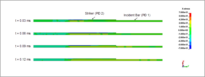
Figure 365 below shows the y-stress contour plot for the incident bar and striker at different timesteps. The plot illustrates that the compressive stress wave moves through the striker and reflects back during the initial 0.12 ms. Meanwhile, a compressive stress wave propagates through the flange and a tensile stress wave propagates through the incident bar with magnitudes lower than the striker stress.
To validate the model and verify the accuracy of the LS-DYNA explicit solver, the magnitude and duration of the first tensile stress wave transmitted through the incident bar resulting from the simulation were compared to the analytical solution. For this purpose, an element located at 1,000 mm from the impact surface (y-coordinate) in the incident bar is used to track the variation of y-stress and calculate the wave magnitude and period. Figure 366 shows the y-stress (GPa) for the bar element versus time (ms).
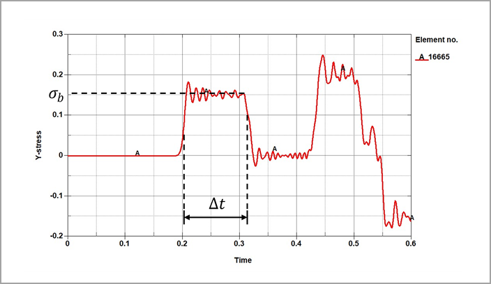
To quantify the error between the analytical and LS-DYNA solutions, the magnitude and period of the first tensile stress wave and their relative errors are calculated in the following results table. For the LS-DYNA model, the stress magnitude is calculated by averaging the stress values between the first and last local peaks of the stress wave. The time period is calculated between two points located in the middle of the pulse rise and fall. As shown in the results table below, the average stress magnitude is calculated as 0.1518 ± 0.0097 GPa, and the wave is experienced during 0.1160 ms. The results show excellent agreement with the analytical solution.
| Results | Target | LS-DYNA Solver | Error (%) |
|---|---|---|---|
Magnitude ( ) of the first tensile elastic stress wave (GPa) ) of the first tensile elastic stress wave (GPa) | 0.1518 | 0.1522 | 0.26 |
Time period ( ) of the first tensile elastic wave (ms) ) of the first tensile elastic wave (ms) | 0.1156 | 0.1160 | 0.28 |