VM-LSDYNA-IMPACT-001
VM-LSDYNA-IMPACT-001
Normal Collision of a Rubber Sphere with a Steel Plate
Overview
| Reference: | Wang, Y., Luo, Z., Wang, H., Zhou, X., Wang, H., & Chen, S. (2025). Characteristics of contact force for normal collision of rubber sphere with rigid plate. AIP Advances, 15(2), 025104. https://doi.org/10.1063/5.0246600 |
| Analysis Type(s): | Explicit Impact Dynamics |
| Element Type(s): | 3D Solid Elements |
| Input Files: | Link to Input Files Download Page |
Test Case
The finite element simulation presented in this test case models the normal collision of a deformable rubber sphere with a rigid steel plate to verify the accuracy of the LS-DYNA explicit solver.
The predicted coefficients of restitution (COR) for three drop heights resulting from the simulation are compared with measured values reported in the literature for identical impact scenarios.
The table below provides the geometric and material properties of the elements used in the test case, as well as loading and boundary conditions. Note that all nodes at the bottom of the rigid plate were constrained to prevent motion during and after impact.
| Material Properties | Geometric Properties | Loading |
|---|---|---|
|
Plate: Density = 7850 kg/m3 Poisson's ratio = 0.3 Young's modulus = 200 GPa
Sphere: Density = 1150 kg/m3 Poisson's ratio = 0.49 C10 = 0.598 MPa C01 = 0.1495 MPa G1 = 10 MPa β1 = 920 (s-1) |
Plate: Thickness = 20 mm Area = 80 mm × 80 mm
Sphere: Diameter = 60 mm |
Impact Velocity by Drop Height: 0.2 m → 1.8254 m/s 0.4 m → 2.6935 m/s 0.8 m → 3.8859 m/s
Boundary Conditions: Plate's bottom nodes are fixed Gravity |
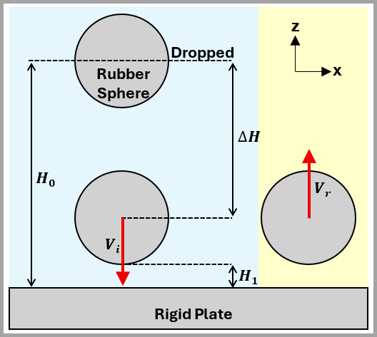
During the simulation, the sphere is released a short distance from the rigid surface (see  = 0.01 mm in Figure 349 below) instead of the actual drop height (for example,
  = 0.8 m). The simulation then imposes an initial velocity (
 ) to replicate that of the sphere after falling the effective drop height (
 ), assuming air resistance is negligible.
 is determined using the following formula, with
  representing the sphere’s radius:
 | (110) |
Figure 349 displays a schematic and imposed velocities ( ) at the drop heights simulated in the test case.
Figure 349: Test Case Schematic and  for Simulated Drop Heights
| Drop Height (m), | Impact Velocity (m/s), |
|---|---|
| 0.2 | 1.8254 |
| 0.4 | 2.6935 |
| 0.8 | 3.8859 |
Analysis Assumptions and Modeling Notes
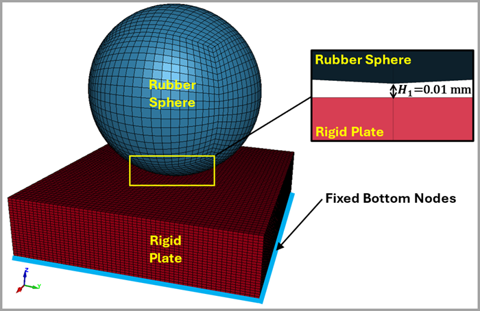
In this model, the entire geometry is discretized using hexahedral solid elements (ELFORM = 1). The simulation uses the SI unit system (N, m, kg, s), but you may adapt the simulation to other systems as needed. Thermal effects are ignored, assuming a constant temperature, as well as surface adhesion or other complex surface phenomena.
The rubber sphere is defined using *MAT_HYPERELASTIC_RUBBER (MAT_077_H), a material that is nearly incompressible with a density of 1150 kg/m3 and Poisson’s ratio of 0.49.
To model the hyperelastic response, a second-order Mooney-Rivlin strain energy function is used with the coefficients C10 = 598,000 Pa and C01 = 149,500 Pa. All higher-order terms are set to zero.
A viscoelastic shear modulus of G1 = 1E7 Pa and decay constant of β1 = 920 s−1 are included to capture damping effects during impact. Failure criteria or thermal effects are not specified.
The rigid plate is defined using *MAT_RIGID (MAT_20), which represents an idealized rigid body with no deformation under load. The density is set to 7850 kg/m3, corresponding to typical steel.
An elastic modulus of 2E11 Pa and a Poisson’s ratio of 0.3 are specified, but because the solver effectively ignores these mechanical properties, the plate is understood to be non-deformable.
To suppress non-physical hourglass deformation modes in the rubber sphere, an hourglass control is also applied using Type 6 (Belytschko-Binderman) with a scaling coefficient QM = 1.0.
The contact interaction between the rubber sphere and the rigid plate is modeled using *CONTACT_AUTOMATIC_SURFACE_TO_SURFACE, a keyword that defines surface-to-surface contact with automatic detection and enforcement.
Because the simulation focuses on normal impact behavior rather than tangential effects, the coefficient of friction is set to zero.
Results Comparison
The table below demonstrates that the simulation accurately predicts the COR values represented in the literature for identical impact scenarios.
| Results | Target | LS-DYNA Solver | Error (%) |
|---|---|---|---|
| COR ( = 0.2 m) | 0.5912 | 0.6064 | 2.57 |
| COR ( = 0.4 m) | 0.6399 | 0.6252 | -2.30 |
| COR ( = 0.8 m) | 0.6619 | 0.6458 | -2.43 |
Note, the simulation aimed to replicate the experimental COR values. A single viscoelastic branch was employed (defined by G1 and β1), a strategy found to be sufficient for capturing the rubber sphere’s energy dissipation during impact. You may employ additional branches to extend the model’s applicability across a broader range of impact velocities or enhance the accuracy of other response variables, such as local deformation.
The figures below include visualizations from the = 0.2 m test case:
The sphere’s rebound speed is tracked using its rigid body velocity in the Z direction. This velocity represents the net translational motion of the entire body, ignoring internal deformation. It reflects a mass-weighted average of all nodal velocities, effectively showing how the object moves as a whole.
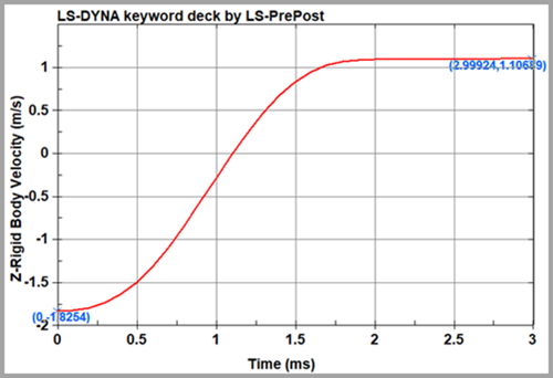
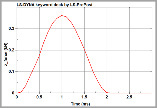
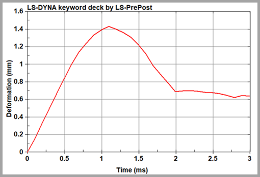
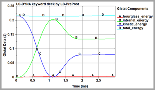
Figure 354 below displays the evolution of energy during the impact scenario. The total energy remains constant, indicating energy conservation and numerical stability. The kinetic energy decreases as the sphere impacts the plate while the internal energy increases, reflecting energy transfer during deformation. Then the kinetic energy rises after the sphere reaches peak deformation and rebounds, though not to its initial value. This pattern is consistent with material damping and energy dissipation. The hourglass energy remains negligible, confirming minimal numerical artifacts.