


The adaptive sizing is an exclusive FreeFlow feature. The SPH Adaptive Sizing Method's main purpose is to give better performance in certain problems, specially for those which is necessary to have a better physical evaluation in a portion of the physical domain, instead of analysing the entire domain. In such cases, it is interesting to have refined elements just near the region of interest instead of refining all SPH elements. Therefore, using the SPH Adaptive for creating refined SPH elements, can lower the computation time.
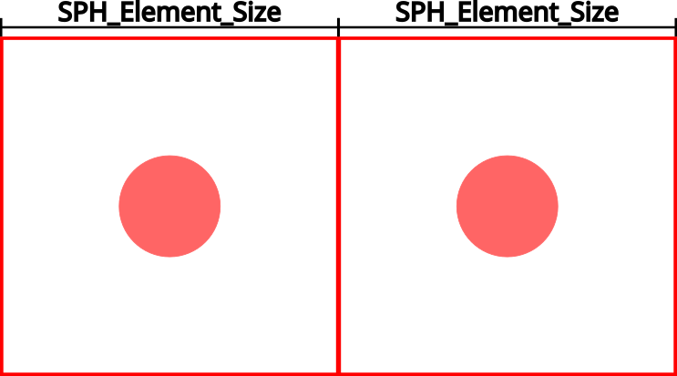
To illustrate how the SPH algorithm works, we will use as example a 2D SPH element refinement. Consider that we want to refine the two bidimensional SPH elements shown in Figure 2.1: Initial SPH elements.. We set the initial SPH Element Size, they are generated, then they will be placed as in Figure 2.1: Initial SPH elements.. Initially, the space reserved for each SPH element is the red square area, in other words, each initial two SPH elements occupies an area equal to SPH Element Size times SPH Element Size. Besides that, the distance between them will also be equivalent to SPH Element Size.
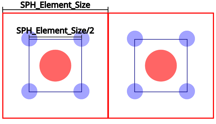
If we set the refinement level to 1, the refined SPH elements will have a size equals to SPH Element Size/2. Thus, each new refined SPH Elements will occupy a square with area equal to SPH Element Size/2 times SPH Element Size/2. Consequently, to conserve the distance between SPH elements, it will be necessary to create new 4 SPH elements, each one occupying a quarter of area of the original one. Also, the total area will be remain unaltered as well, i.e., the sum of the area of each element will be the same as of the original element. The placement of the new SPH elements is illustrated in Figure 2.2: Representation of refined and non-refined SPH elements with refinement level equal to 1. The red circles represent original elements and the blue ones represent the refined ones.
In a general form, we can say that the following equation,
 | (2–1) |
where n is the Refinement Level, gives the size of the refined SPH elements and the new distance among the refined SPH Elements.
In a similar manner, for 2-D elements the area will be reduced by
 | (2–2) |
and for 3-D elements the volume will be reduced by  .
.
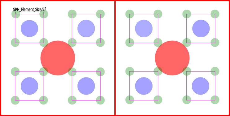
Consider Equation 2–1 and Equation 2–2, one can say that if the user sets a refinement level equal to 2, the distance between each SPH Element will be reduced by 4, if refinement is equal to 3, the distance will be reduced by 8 and so on. Then, if we set a refinement level equal to 2, the original area will be reduced by 16. Consequently, we will need to create 16 new SPH elements to maintain the area and distance between elements. In Figure 2.3: Representation of two types of refined SPH elements (green and blue) and non-refined elements (red) alongside the original element (red), and the element refined with level equal to 1 (blue), there is also a refined element with level equal to 2 (green).
Figure 2.3: Representation of two types of refined SPH elements (green and blue) and non-refined elements (red)
In Ansys FreeFlow there is a slight difference between the algorithm explained before, SPH Adaptive Sizing Method Overview, and what was implemented. As Ansys FreeFlow is a 3D software, the refinement algorithm is performed using as reference a cube, instead of a square. Equally, the cube centered in the element to be refined and the initial cube has a side length of a SPH Element Size. Once the refinement process is activated and performed, the new SPH elements (refined ones) will be inserted in the vertices of a new cube, which side length is equal to the division of the initial SPH size by the Refinement level.
There are also other characteristics in Ansys FreeFlow implementation. The process
of refining occurs at every 20 solver iterations and it is constant during all the
simulation, i.e., the user can not change it. Besides that, the
refinement process will be performed if two conditions are satisfied. The first one
concerns with the Refinement Count value, an SPH element is
refined if its Refinement Count value is lower than
 , where n stands for Refinement Level. The
second condition for an SPH element to be refined is its location, if the SPH
Element is inside a refinement region, the refinement is done, otherwise the element
remains unaltered.
, where n stands for Refinement Level. The
second condition for an SPH element to be refined is its location, if the SPH
Element is inside a refinement region, the refinement is done, otherwise the element
remains unaltered.
Moreover, Figure 2.2: Representation of refined and non-refined SPH elements with refinement level equal to 1 shows, just as reference, all the SPH elements, refined and non-refined SPH elements. In a real simulation, all the red elements (non-refined) will be excluded. Also, it is important to remind you that on Ansys FreeFlow all SPH elements will be represented by pixels of the same length, independently of its size. In order to see the refined elements, one can plot the Refinement Count property.
At Ansys FreeFlow there are two main ways to use the adaptive sizing, i.e., to determine the refinement region. One is by choosing boundary proximity as reference or by using ROIs. A combination of both is also possible, in the next two sections the details about both approaches are shown.