The following sections of this chapter are:
The Fluent Discrete Phase Model (DPM) can be used to simulate droplets flow in the Fluent Icing workspace as an alternative to the default Particles solver based on a FENSAP™ legacy solver (DROP3D). The Discrete Phase Model is based on the Lagrangian tracking of particle streams whereas the default solver is based on an Eulerian formulation. Fluent Icing uses the steady DPM solver which tracks the permanent particle flow rate on the particle trajectories. More information regarding the details of the steady DPM solver can be found in (Discrete Phase). This chapter describes how to enable Discrete Phase Model and how to setup the injection properties and the physical models.
Only droplets can be resolved. Ice crystal icing and vapor are not supported in the current version.
Only planar inlet surfaces must be used to inject discrete particles.
The interaction between the continuous phase and the Lagrangian phase is one-way.
To enable the DPM solver for Particles in Fluent Icing, perform the following steps:
Enable .
 File
→ Preferences...
→ Icing → Beta
Features
File
→ Preferences...
→ Icing → Beta
Features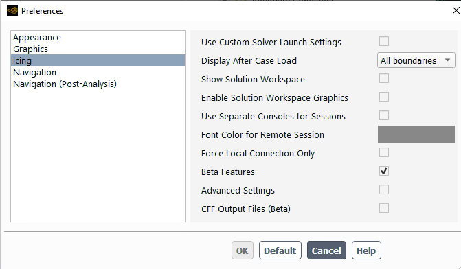
Set up the Particles properties of your simulation.
 Setup →
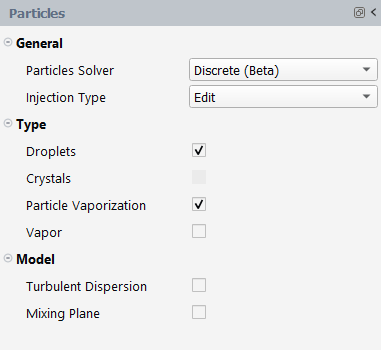
After enabling , a Particles Solver drop-down list is activated in the Particles window. By default, the solver is selected, which corresponds to the usual feature described in Particles.
Under the General section, retain the following setting:
for Particles Solver.
for Injection Type.
Note: When using the discrete phase model, particles are released from a given set of point locations and their trajectories are tracked until they reach a final fate (trapped, escaped). Therefore, you need to provide injection properties including initial conditions, as well as boundary interaction properties.
: Injections are explicitly defined by you in the Fluent case file following the instruction given in Setting Initial Conditions for the Discrete Phase. The injection’s name should not start by
flicing-drop-, or it will be ignored by the solver as the name is reserved for the option.: Injections are automatically created from the Fluent Icing interface at inlet boundary conditions (pressure inlet, velocity inlet, mass flow inlet or pressure far field).
When is activated, the Airflow solver is automatically set to and only the Droplets object remains in the Outline View under
Setup → Under the Type section, retain the following settings:
Enable to assign droplets properties to the particles. Disabling will automatically select the option and crystal properties will be assigned to the particles.
Enable to account for the particle mass loss due to vaporization.
Enable to solve the vapor Eulerian field when is enabled.
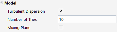
Under the Model section, retain the following settings:
Enable the model for DPM. Only the discrete random walk model is available in Fluent Icing. This model is described in The Integral Time.
Note: When the model is activated, the Number of Tries must be specified.
Enable to enable the particles mixing plane statistics computation at the outlet boundary conditions and/or mixing plane profiles reinjection at inlet conditions.
Note: When is activated, the Mixing Plane Number of Bands and Mixing Plane Distribution Percentiles must be specified. The Mixing Plane Inlet File can be specified to use a profile for particle properties.
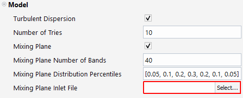
The Mixing Plane Number of Bands corresponds to the number of bands generated based on the outlet boundary conditions selected for mixing plane data collection. The minimum and maximum radial coordinates are extracted from the subset of outlet conditions selected and regular bands are generated based on those coordinates. During the DPM resolution, the Lagrangian properties are collected at the mixing plane outlet condition and stored by band and by diameter bins of 1 micron width.
The Mixing Plane Distribution Percentiles is used to determine the diameters of the particle distribution reaching the outlet conditions for the selected outlet conditions. Each percentile corresponds to the mass flow rate percentage of the particles reaching the outlet, with increasing particle diameter. Then the mixing plane algorithm will reconstruct the flow rate and all the particle properties of those diameters for every individual band of the mixing plane, to finally obtain a profile of the quantities for each diameter of the distribution. An output file is automatically generated at the run level with the .mpdat extension. This file contains the profile information for the distribution.
Note: The constraint for the profile reconstruction is based on the diameters of the particle rather than the mass of the percentiles. Starting from the smaller bins, the whole mass of the bins is accumulated until the averaged value of the diameter reaches the diameter of the outlet distribution. Then, the algorithm switches to the next distribution diameter, and the same process is repeated until all the distribution diameters mass flow rates are known for every bands.
Select a Mixing Plane Inlet File to inject a radial profile of particle properties for a number of diameters specified in the file. This file can be generated by a mixing plane calculation performed on a previous stage for a Turbomachinery simulation. When a file is selected the physical inlet boundary condition parameters defined in the graphical user interface are not used for the particles and for the vapor. You still have to specify the two following fields at the boundary level to create the injection:
Use for injection
Number of streams
Set up the Droplets properties of your simulation.
Setup → → 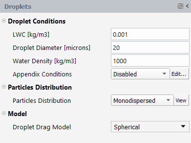
When Droplets is selected in the Outline View under
Setup → ,
the Droplets window appears. In this window, you can
specify the ambient/reference conditions of the water droplets, the type and
size distribution, and some physical models.In the Droplet Conditions section, the parameters describing the droplets are:
LWC [kg/m3]: Reference liquid water content (LWC) which can be used either for collection efficiency normalization or for injection properties.
Droplet Diameter [microns]: Median volume diameter (MVD) of a spherical particle for a given distribution which is used only when is used to create injections.
Water Density [kg/m3]: Density of water droplets.
In the Particles Distribution section, the distribution type can be selected when using to create injections. The available distributions are those described in Particles:
.
to .
.
Appendix Conditions are not available with the discrete particles solver.
For particle distributions, the Fluent DPM model will solve the particle tracks for every given diameter, then the final Eulerian solution is obtained by averaging the single diameter solutions using the weights of the size distribution.
Note: When is enabled, all particles are solved in a single calculation and only the final Eulerian solution is available.
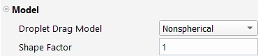
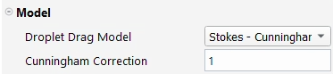
In the Model section, the appropriate Droplet Drag Model can be selected:
: No additional changes are needed.
: Specify the .
: Specify the Cunningham Correction.
: Click the button to update the list of available user-defined functions loaded in the Fluent case file. The user-defined functions listed should be generated using the
DEFINE_DPM_DRAGmacro (Discrete Phase Model (DPM)DEFINEMacros).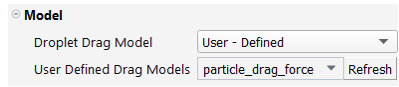
Set up the Crystals properties of your simulation.
Setup → Particles → 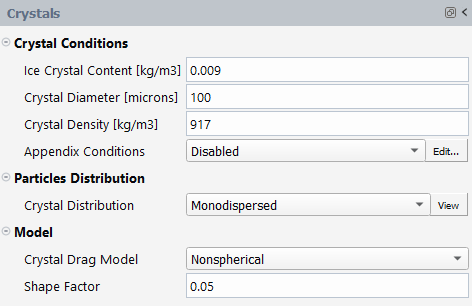
When Crystals is selected in the Outline View under
Setup → Particles
The Crystals panel appears. Within it, you can specify
the ambient/reference conditions of the crystals, the type and size
distribution, and physical models. In the Crystal
Conditions section, the parameters representing the droplets
are:Ice Crystal Content [kg/m3]: Reference ice crystal content (ICC) which can be used either for collection efficiency normalization or for injection properties.
Crystal Diameter [microns]: Median volume diameter (MVD) of a spherical particle for a given distribution which is used only when
Setup → Particles → → is used to create
injections.Crystal Density [kg/m3]: Density of crystals.
In the Particles Distribution section, the distribution type can be selected when using
Setup → Particles → → to create injections. The
available distributions are or
.Note: Appendix Conditions are not available with the discrete particles solver.
For particle distributions, the Fluent DPM model will solve the particle tracks for every given diameter, then the final Eulerian solution is obtained by averaging the single diameter solutions using the weights of the size distribution.
Note: When Vapor is enabled, all the particles are solved in a single calculation and only the final Eulerian solution is available.
In the Model section, the appropriate Droplet Drag Model can be selected:
: No additional changes are needed.
: Specify the .
: Click the button to update the list of available user-defined functions loaded in the Fluent case file. The user-defined functions listed should be generated using the
DEFINE_DPM_DRAGmacro (Discrete Phase Model (DPM)DEFINEMacros).
Set up the inlet Boundary Conditions of your simulation.
Setup → Boundary
Conditions → → → The discrete phase model requires initial droplet or crystal properties definition at their injection points location. Fluent Icing will use Inert Particles type (consult Particle Types) as only momentum and heat will interact with the carrier phase. For Inert Particles type, the properties include the stream flow rate, velocity components and temperature. In Fluent Icing, with the injection mode enabled, Particles can be released from inlet boundary conditions surfaces. To this end, surface injections are automatically created for every chosen inlet conditions and the Randomize Starting Point option which is automatically selected leads to a uniform distribution of the injection points on this surface.
Droplets Inlet Boundary Conditions
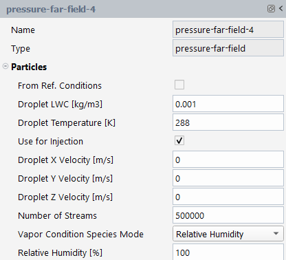
From Ref. Conditions: If enabled using the discrete particles solver, only the reference LWC and temperature are used.
Droplet LWC [kg/m3]: If From Ref. Conditions is unchecked, set the water droplet concentration.
Droplet Temperature [K]: Specify the temperature of the cloud of water droplets at the inlet.
Use for Injection: Enables the creation of a new injection based on the boundary condition surface.
Droplet X,Y,Z Velocity [m/s]: Sets the velocity components of the water droplet cloud.
Crystals Inlet Boundary Conditions
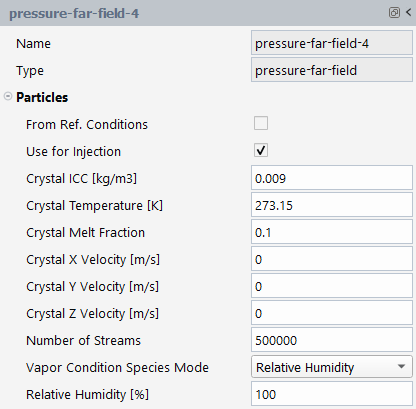
From Ref. Conditions: If enabled using the discrete particles solver, only the reference ICC and temperature are used.
Crystal ICC [kg/m3]: If From Ref. Conditions is unchecked, set the ice content concentration.
Crystal Temperature [K]: Specify the temperature of the cloud of water droplets at the inlet.
Crystal Melt Fraction: A value between 0 and 1 can be assigned if the crystal temperature is equal to 273.15K. For a crystal temperature lower or greater than 273.15K, the melt fraction is automatically set to 0 and 1, respectively.
Crystal X,Y,Z Velocity [m/s]: Sets the velocity components of the ice crystal cloud.
General Particles Inlet Boundary Conditions
: Enables the creation of a new injection based on the boundary condition surface.
Number of Streams: Numerical parameters, defines the number of points located at the surface releasing a particle stream.
Vapor Inlet Boundary Conditions
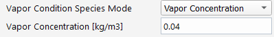
Vapor Condition Species Mode: Choose between , or for the vapor inlet boundary condition specification.
Relative Humidity [%]: Set the inlet relative humidity value.
Vapor Concentration [kg/m3]: Set the inlet vapor concentration value.
Select the wall boundary condition for the particles
Setup → Boundary
Conditions → → → 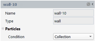
: The particles are collected locally when hitting the wall ending the particle trajectory. The particle fate is listed as Trap in the summary.
: The particles are reflected when hitting the wall. The rebound velocity vector is in the same plane as the incident velocity vector and the wall normal vector. The components are computed using normal and tangential rebound coefficients. The Normal and Tangential rebound coefficients
 are defined as polynomes of the impact angle
θ (in degree):
are defined as polynomes of the impact angle
θ (in degree):Where
 is the polynomial coefficient in direction
  to be defined.
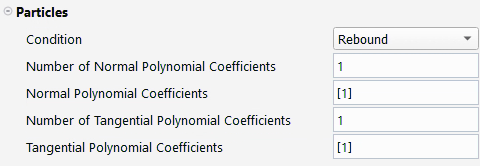
Number of Normal Polynomial Coefficients: Sets the number of polynomial coefficients (1 to 8) for the normal rebound coefficient. The Normal Polynomial Coefficients field will be automatically updated.
Normal Polynomial Coefficients: Sets the value of the polynomial coefficients for the normal component of the velocity. The coefficient must be positive.
Number of Tangential Polynomial Coefficients: Sets the number of polynomial coefficients (1 to 8) for the tangential rebound coefficient. The Tangential Polynomial Coefficients field will be automatically updated.
Tangential Polynomial Coefficients: Sets the value of the polynomial coefficients for the tangential component of the velocity.
: Mundo formulation is used to evaluate the local collection of particles. When a particle stream impacts the wall, it will either splash or be reflected depending on the impact and particle properties. When the particle stream splashes, part of the mass is collected at the wall and the remaining mass is reinjected using rebound coefficients and a diameter computed by the Mundo model (Mundo Model).
: Click the button to update the list of available user-defined functions loaded in the Fluent case file. The user-defined functions listed should be generated using the
DEFINE_DPM_BCmacro (Discrete Phase Model (DPM) DEFINE Macros). The function should update the particle stream properties including velocity components, droplet diameter and flow rate. The change in flow rate after impingement will be automatically collected locally at the wall. Some variables might need an update of the value entering the cell and of the initial value. Table 39.3: List of Variables to Update in DEFINE_DPM_BC Macro provides the list of variables to update in the UDF.Table 39.3: List of Variables to Update in DEFINE_DPM_BC Macro
Velocity ith component [m/s] TP_VEL(tp)[i] and TP_VEL0(tp)[i] Droplet mass [kg] TP_MASS(tp), TP_MASS0(tp) and TP_MASS_INIT(tp) Droplet diameter [m] TP_DIAM(tp), TP_DIAM0(tp) Stream flow rate [kg/s] TP_FLOW_RATE(tp) Example:
This example shows the usage of
DEFINE_DPM_BCfor the fragmentation of crystals when they hit the walls. The function assumes that the mass of a single particle after the collision is 30% of the impinging particle mass (fragmentation_coeff = 0.3) and the flow rate is equal to 50% (sticking_coeff = 0.5) of the incoming flow rate (which means that 50% of the incoming flow rate is collected at the wall). For the crystals reinjected in the airflow, the function assumes an ideal reflection for the normal component of the velocity (nor_coeff = 1.) while the tangential component is damped (tan_coeff = 0.3). The function returnsPATH_ACTIVEfor the crystals reinjected in the airflow while it stops all other particles returningPATH_ABORT.#include "udf.h" #define PART_MIN_DIAMETER 1.e-6 DEFINE_DPM_BC(bc_sticking_fragmentation,tp,t,f,f_normal,dim) { real vn=0.; real nor_coeff = 1.; real tan_coeff = 0.3; real fragmentation_coeff = 0.3; /* particle diameter ratio after and before wall impingement*/ real sticking_coeff = 0.5; /* mass fraction accumulated at the wall */ int i; /* DPM Types used in Fluent Icing - 3D only */ if(TP_TYPE(tp) == DPM_TYPE_INERT || TP_TYPE(tp) == DPM_TYPE_DROPLET) { /* calculate the normal component, rescale its magnitude by the coefficient of restitution and subtract the change */ /* Compute normal velocity. */ for(i=0; i<dim; i++) vn += TP_VEL(tp)[i]*f_normal[i]; /* Subtract off normal velocity. */ for(i=0; i<dim; i++) TP_VEL(tp)[i] -= vn*f_normal[i]; /* Apply tangential coefficient of restitution. */ for(i=0; i<dim; i++) TP_VEL(tp)[i] *= tan_coeff; /* Add reflected normal velocity. */ for(i=0; i<dim; i++) TP_VEL(tp)[i] -= nor_coeff*vn*f_normal[i]; /* update individual particle mass TP_MASS update TP_INIT_MASS too to evaluate the number of particles */ TP_MASS(tp)*=fragmentation_coeff; TP_INIT_MASS(tp)=TP_MASS(tp); /* compute new individual particle diameter */ TP_DIAM(tp)=pow(6.*TP_MASS(tp)/TP_RHO(tp)/M_PI,1./3.); /* update stream flow rate */ TP_FLOW_RATE(tp)*= (1. - sticking_coeff); /* Update particle state variables at cell entry */ for(i=0; i<dim; i++) TP_VEL0(tp)[i] = TP_VEL(tp)[i]; TP_MASS0(tp)=TP_MASS(tp); TP_DIAM0(tp)=TP_DIAM(tp); if (TP_DIAM(tp)>PART_MIN_DIAMETER) return PATH_ACTIVE; else return PATH_ABORT; } return PATH_ABORT; }
Select the outlet boundary conditions under Particles.
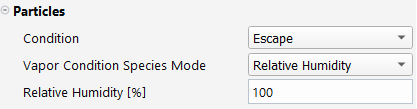
Condition: If is enabled, choose between a regular condition for particles, or a condition which is an escape condition coupled with data collection for mixing plane statistics computation. If is not enabled, this option does not appear and a regular escape condition is always applied.
Vapor Condition Species Mode: Choose between Relative Humidity, Vapor Concentration or Case Settings for the vapor outlet boundary condition specification for reverse flows.
Relative Humidity [%]: Set the outlet relative humidity value for reverse flows.
Vapor Concentration [kg/m3]: Set the outlet vapor concentration value for reverse flows.
There is nothing more to set up for the other boundary conditions.
At the outlet boundary conditions, particles will escape the domain.
At the symmetry conditions, particles will be reflected.
For periodic boundaries, particles are re-injected at the associated face when leaving the domain using the transformation matrix of the periodic boundaries (position, velocity).
Set up the discrete phase solver numerical settings.
Solution → Particles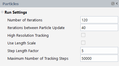
Number of Iterations: When is enabled, set the number of iterations for vapor resolution.
Iterations between Particle Update: When is enabled, this option lets you set the number of vapor iterations between two calculations of the particle trajectories and the update of the vapor source terms resulting from the particle resolution.
: If enabled, accuracy of the tracking is improved by using the subtet approach, see High-Resolution Tracking under Tracking Settings for the Discrete Phase Model.
:
If enabled, a user-defined can be used for tracking.
If disabled, the step length scale is based on the local mesh size, and a can be applied to subdivide the maximum tracking time step.
Maximum Number of Tracking Steps: For each stream, the Lagrangian particle tracking ends up by reaching its final fate (escaped, trapped) or if this number of tracking time step is reached (incomplete fate).

Displaying discrete variables for the last particle only.
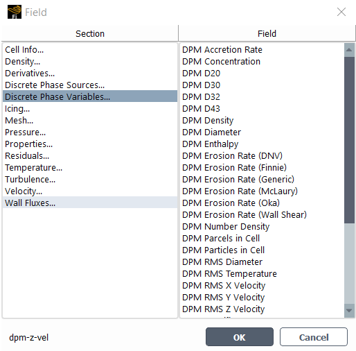
Results → Contours New...
Click within the Field box.
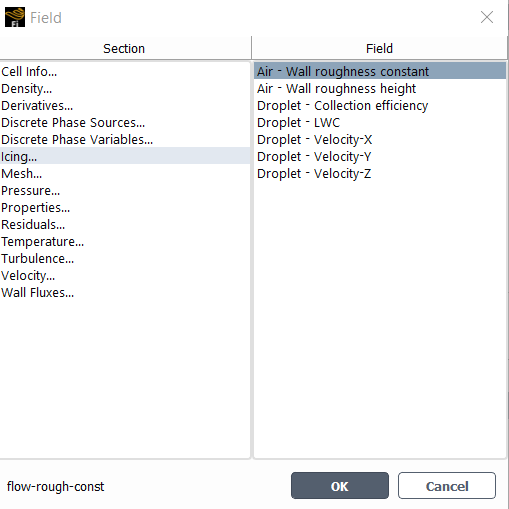
Discrete phase variables are available for display for the last particle tracking only, by selecting Discrete Phase Variables… under the Field dialog.
Icing quantities in Icing… under the Field dialog are derived from Discrete Phase Variables… quantities. Distribution will contain the combined solution of Droplet – LWC, Velocity components and Collection efficiency.
The Droplet – Collection efficiency β is obtained by normalizing the DPM Accretion Rate
 :
:With:
 the reference liquid water content LWC
[kg/m3] specified in the Droplets
panel.
the reference liquid water content LWC
[kg/m3] specified in the Droplets
panel. the reference Speed [m/s]
specified in the Airflow panel.
the reference Speed [m/s]
specified in the Airflow panel.

This tutorial is divided into the following sections:
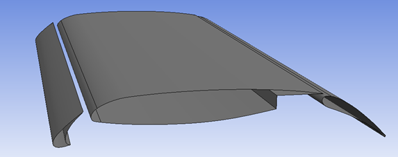
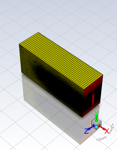
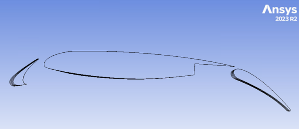
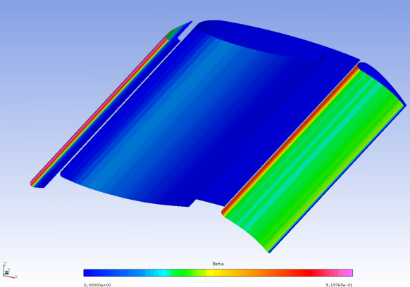
In the following tutorial, you will learn how to use the Discrete Phase Model, as an alternative to DROP3D, to solve the droplets flow for icing simulations. The example is based on the geometry shown below, which is an airfoil composed of three elements.
This tutorial is written with the assumption that you have reviewed the material above and have familiarized yourself with the details of the steady DPM solver in (Discrete Phase). Some steps in the setup and solution procedure will not be shown explicitly.
This is an ice accretion simulation on a multi-element airfoil with the slat and the flap deployed. The mesh type is 2.5D, meaning that a surface mesh generated on the periodic source face of the domain is extruded with a single cell in the direction of the extrusion. It allows you to select the 2.5D remeshing technique. The airfoil is placed inside a wind-tunnel test section enclosure instead of a far field boundary. The angle of attack is 4 degrees, which is built in to the computational model since the airfoil is situated inside the test section.
The following sections describe the setup and solution steps for this tutorial:
To prepare for running this tutorial:
Download the fluent_icing_three_element_dpm_multishot.zip file here .
Unzip fluent_icing_three_element_dpm_multishot.zip in your working directory.
The files 3element_airfoil_1.cas.h5 and 3element_airfoil_1.dat.h5 can be found in the folder.
Launch Fluent 2025 R2 on your computer.
Within the Fluent Launcher, set the Capability Level to CFD Enterprise, then select Icing.
Set Solver Processes to
8under Parallel Processing Options.Click Start.
Alternatively, Fluent Icing can be opened using the icing (on Linux) or icing.bat (on Windows) file inside the fluent/bin/ folder.
Uncheck , , and .
Project
→ Workspaces → Options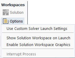
Create a new project file.
File → New
Project... Enter
three_element_airfoilas the Project file name within the Select File dialog.Select and import the 3element_airfoil_1.cas.h5 input grid.
Project
→ Simulation → Import
Case A New Simulation window will appear. Enter the Name of the New Simulation as
3element_airfoil_1, and check to enable and . Click .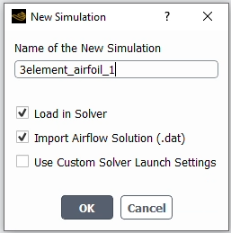
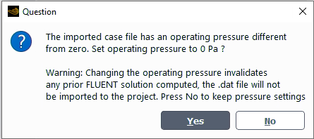
A dialog will open asking you to set the operating pressure to 0 Pa. Press to keep pressure settings.
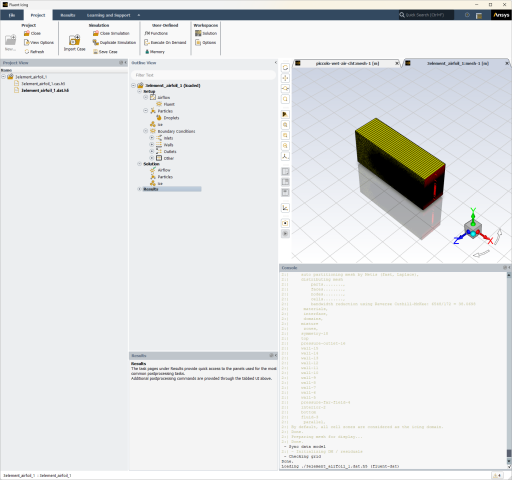
After the .cas.h5 file has been successfully loaded, a new Outline View tree appears under 3element_airfoil_1 (loaded).
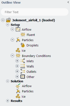
The mesh is now displayed in the Graphics window to the right.
Enable to expose features that are not yet fully supported.
File
→ Preferences... →
Icing → Define the Simulation Type.
Setup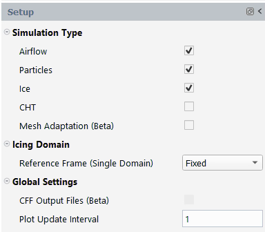
Enable , and Simulation Type within the Setup panel.
Set the Airflow properties for the simulation.
Setup → Airflow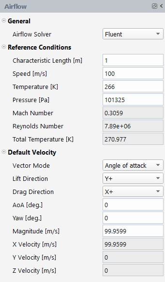
In the General section:
Retain the default selection of for Airflow Solver.
In the Reference Conditions section, retain the following settings:
1for Characteristic Length [m].100for Speed [m/s].266for Temperature [K].101325for Pressure [Pa].
In the Default Velocity section, set the following settings:
for Vector Mode.
for Lift Direction.
for Drag Direction.
0for AoA [deg.]. The airfoil is already at a 4-degree angle of attack with respect to the X-coordinate and tunnel walls. The flow into the test section is specified without an angle of attack.0for Yaw [deg.].99.9599for Magnitude [m/s].
Set the Particles properties of the simulation.
Setup → Particles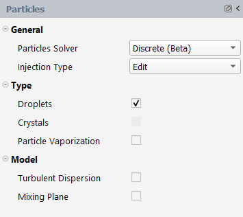
In the General section, retain the following settings:
for Particles Solver.
for Injection Type.
In the Type section, retain the following settings:
Enable Droplets.
Note: Crystals will automatically be selected.
Set the Droplets properties of the simulation.
Setup → Particles → Droplets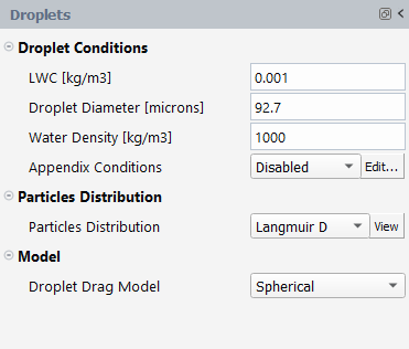
In the Droplet Conditions section, retain the following settings:
0.001for LWC [kg/m3].92.7for Droplet Diameter [microns].1000for Water Density [kg/m3].for Appendix Conditions.
In the Particles Distribution section, retain the following setting:
for Particles Distribution and press to display the distribution.
In the Model section, retain the following setting:
for Droplet Drag Model.
Disable .
Set the Ice properties of the simulation.
Setup → Ice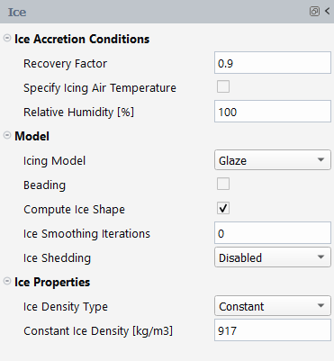
In the Ice Accretion Conditions section, retain the following settings:
0.9for Recovery Factor.Disable Specify Icing Air Temperature.
100for Relative Humidity.
In the Model section, retain the following settings:
for Icing Model.
Disable Beading.
Enable .
0for Ice Smoothing Iterations.for Ice Shedding.
In the Ice Properties section, retain the following settings:
for Ice Density Type.
917for Constant Ice Density [kg/m3].
Set the Boundary Conditions of the simulation.
Setup → Boundary
Conditions → Inlets → pressure-far-field-4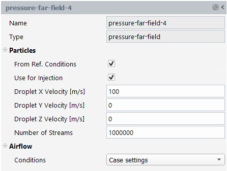
In the Particles section, retain the following settings:
Enable From Ref. Conditions.
Enable Use for Injection.
100for Droplet X Velocity [m/s].0for Droplet Y Velocity [m/s].0for Droplet Z Velocity [m/s].1000000for Number of Streams.
In the Airflow section, retain the following setting:
for Conditions.
Setup → Boundary
Conditions → Walls → wall-5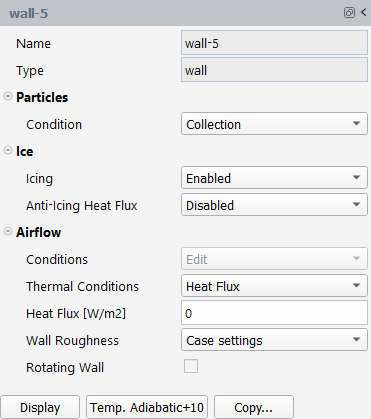
Important: For each wall boundary condition, press on to ensure a temperature value (adiabatic temperature + 10 degree) is imposed.
In the Particles section, retain the following setting:
for Condition.
In the Ice section, retain the following setting:
for Icing.
for Anti-Icing Heat Flux.
In the Airflow section, retain the following settings:
for Thermal Conditions.
276for Temperature [K].for Wall Roughness.
Disable .
Note: Alternatively, the following Python command can be executed in the Console to update every wall thermal boundary condition:
for condName in csim().BC.getState():
 if csim().BC[condName].BCType.getState() == 'wall':
  csim().BC[condName].CopyWallAdiabaticP10()
Set the Solution properties of the simulation.
Solution → Airflow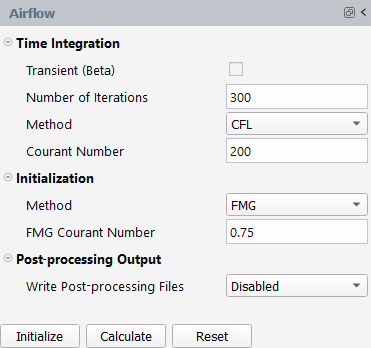
In the Time Integration section, retain the following settings:
300for Number of Iterations.for Method.
200for Courant Number.
In the Initialization section, retain the following settings:
for Method.
0.75for FMG Courant Number.
In the Post-processing Output section, retain the following setting:
for Write Post-processing Files.
Solution → Particles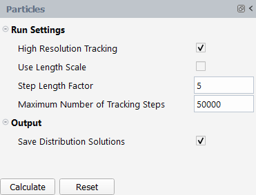
In the Run Settings section, retain the following settings:
Enable .
Disable .
5for Step Length Factor.50000for Maximum Number of Tracking Steps.
Solution → Ice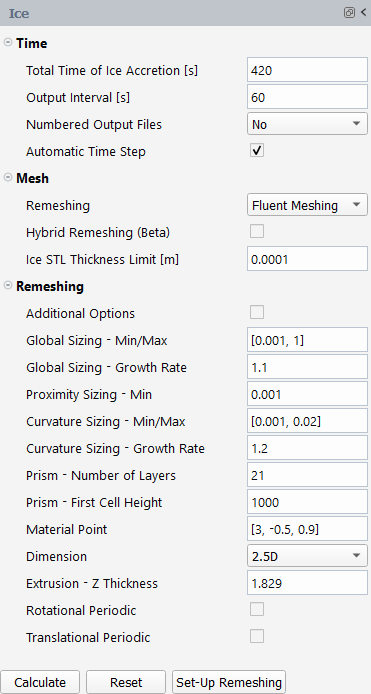
In the Time section, retain the following settings:
420for Total Time of Ice Accretion [s].60for Output Interval [s].for Numbered Output Files.
Enable Automatic Time Step.
Click to display the remeshing settings.
In the Mesh section, retain the following settings:
for Remeshing.
Disable Hybrid Remeshing (Beta).
0.0001for Ice STL Thickness Limit [m].
In the Remeshing section, retain the following settings:
[0.001, 0.1]for Global Sizing - Min/Max.1.1for Global Sizing - Growth Rate.0.001for Proximity Sizing - Min.[0.001, 0.02]for Curvature Sizing - Min/Max.1.2for Curvature Sizing - Growth Rate.21for Prism - Number of Layers.1000for Prism - First Cell Height.[3, -0.5, 0.9]for Material Point.for Dimension.
1.829for Extrusion - Z Thickness.
Launch the simulation.
Solution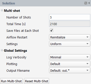
In the Multi-shot section, retain the following settings:
5for Number of Shots.Enable .
for Airflow Restart.
for Settings.
In the Global Settings section, retain the following settings:
for Log Verbosity.
for Plotting.
for Output Filename.
Launch the simulation by pressing .
A New run window will appear. Set the Name of the new run to
multishot_discreteand press .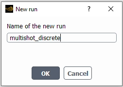
Note: Alternatively, you can launch the multi-shot calculation using
Solution Run
Multi-Shot
Post-process your icing solution.
Project → Project
View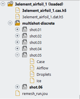
Under the 3element_airfoil_1 (loaded) simulation, a new run named multishot_discrete now appears. Expand the run by clicking the + icon to the left of multishot_discrete to show the files associated with the run. Each shot is represented by a folder and includes a two digit number to specify the shot number. Each folder contains a mesh file (Case), and 3 solution files (Airflow, Droplets and Ice).
Once all calculations are complete, you can view the growth of the ice shape by right-clicking Case located under shot.01 within the Project View. Select → .
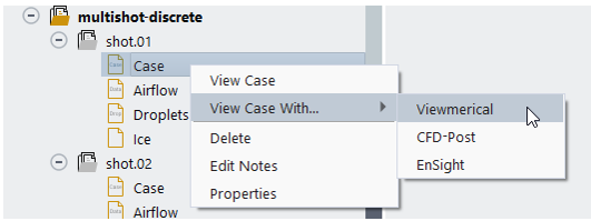
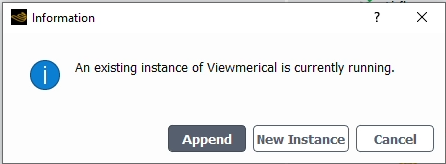
Repeat this procedure for shot.02, shot.03, shot.04, shot.05 and shot.06. Always choose in the Information dialog boxes to keep the current Viewmerical session open.
Within the Viewmerical Objects panel, keep only wall conditions selected. Click the Z-axis in the graphical user interface and to obtain the following figure, showing the growth of the ice shape during the multi-shot simulation.
Close Viewmerical.
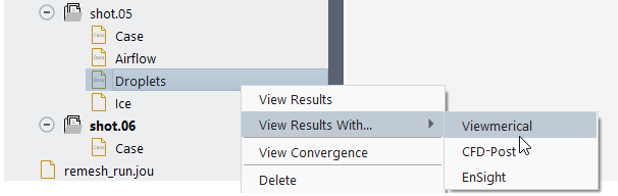
Right-click Droplets under shot.05 in the Project View, and select -> .
In the Objects panel, create a -coordinate Cutting Plane.
In the Data panel, select Data → , choose for the color range and change the upper bound to
0.0015.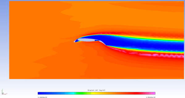
In the Objects panel, keep only wall boundaries selected (BC_2005 to BC_2015).
In the Data panel, select Data → , choose Spectrum-2 – 64 for the color range.
In the Objects panel, select only BC_2009 and BC_2014 to keep the walls of the slat element only.
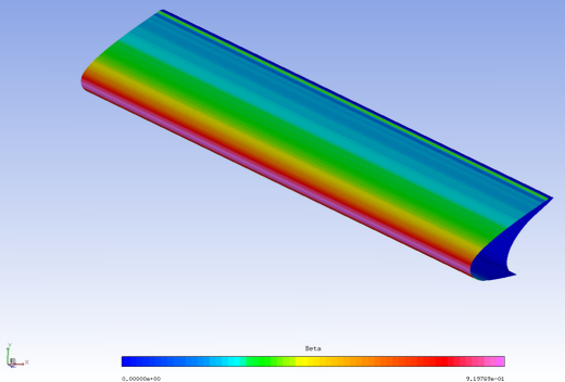
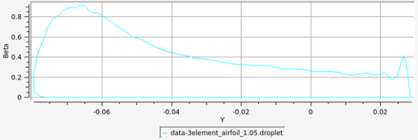
To display the droplet collection efficiency profile on the first element, in the Query panel, choose:
2D Plot: .
Target: .
Cutting plane: .