


The following sections of this chapter are:
This chapter illustrates the procedure for computing Conjugate Heat Transfer (CHT) through the metal skin of the leading edge of a wing heated by electro-thermal pads. The CHT analysis is performed in wet air.
This tutorial is divided into the following sections:
In this tutorial, you will learn how to perform a transient Conjugate Heat Transfer (CHT) analysis on the heated metal skin of the leading edge of a wing.
The analysis will involve the use of electro-thermal pads for de-icing purposes and will be carried out in a wet air environment.
CHT computation contains at least one fluid and one solid domain. The fluid and solid interfaces should be set up in Fluent before importing the case to Fluent Icing. To learn more about setting up the fluid and solid interfaces, consult Non-Conformal Meshes.
Particle trajectory and icing calculations will be carried out in the external flow domain only. Therefore, it is required to indicate which domain is the icing domain in the CHT setup.
The main steps are as follows:
In Fluent, prepare the unheated dry air CHT and get a fully converged solution.
Import the solution into Fluent Icing and launch an initial particles and ice calculation.
Continuing in Fluent Icing, set up a transient de-icing simulation and launch the calculation.
The following sections describe the setup and solution steps for this tutorial:
To prepare for running this tutorial:
Download the fluent_icing_cht.zip file here .
Unzip fluent_icing_cht.zip to your working directory.
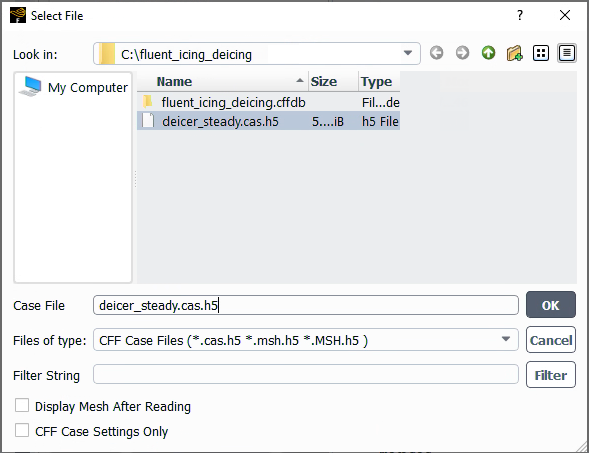
The file, deicer_steady.cas.h5, can be found in the folder.
Launch Fluent 2025 R2 on your computer.
Within the Fluent Launcher, select Solution.
Set Solver Processes to
8under Parallel (Local Machine).Set Dimension to , and Solver Options to Double Precision.
Click Start.
Before launching a transient de-icing simulation, prepare a steady state CHT solution as the initial solution. Read the deicer_steady.cas.h5 case file,
 → →
→ →
Define your solver.
Physics
→ General...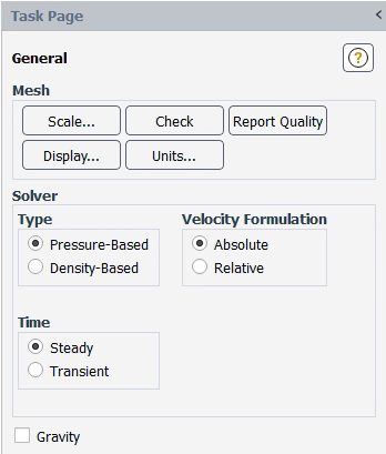
In the General task page, retain the following settings:
for Solver Type.
for Velocity Formulation.
for Time.
Define your operating conditions.
Physics → Solver
→ Operating Conditions...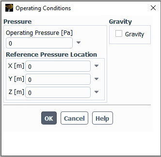
In the Pressure section, retain the following setting:
0for Operating Pressure [Pa].
Set the Fluent properties of the simulation.
 Setup → Models → Viscous
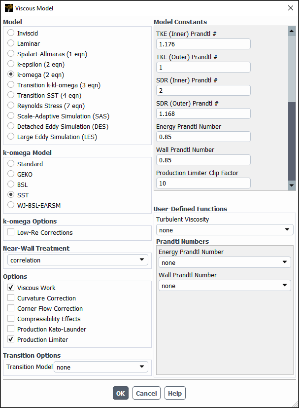
In the Model section, retain the following setting:
for Model.
In the k-omega Model section, retain the following setting:
for k-omega Model.
In the Options section, retain the following settings:
Enable Viscous Work.
Enable Production Limiter.
In the Model Constants section, retain the following settings:
0.85for Energy Prandtl Number.0.85for Wall Prandtl Number.
Enable the Energy Equation.
Setup → Models → Energy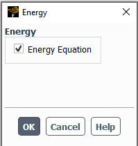
Verify the air properties.
Setup → Material → Fluid → air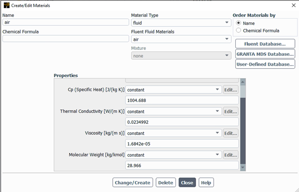
In the Properties section, retain the following settings:
for Density [kg/m3].
1004.688for Cp (Specific Heat) [J/(kg K)].0.0234992for Thermal Conductivity [W/(m K)].1.6842e-05for Viscosity [kg/(m s)].28.966for Molecular Weight [kg/kmol].
Verify the layers of the metal skin. Double-click each one and verify its properties.
Setup → Material → Solid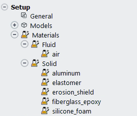
The table below describes the solid properties to be imposed in this simulation.
Name Density [kg/m3] Cp (Specific Heat) [J/(kg K)] Thermal Conductivity [W/(m K)] elastomer 1383.955 1256.04 0.2561 erosion_shield 8025.25 502.416 16.26 fiberglass_epoxy 1794 1570.05 0.294 silicone_foam 648.75 1130.436 0.121 Verify that each corresponding material has been properly assigned.
Setup → Cell Zone
Conditions → Solid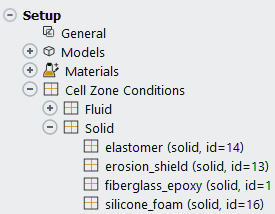
Set up the boundary conditions.
Setup → Boundary
Conditions → Inlet → pressure-far-field-4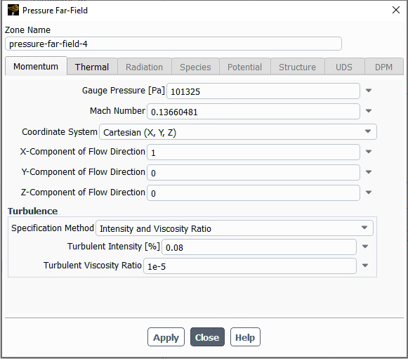
In the Momentum section, retain the following settings:
101325for Gauge Pressure [Pa].0.1366048for Mach Number.1for X-Component of Flow Direction.0for Y-Component of Flow Direction.0for Z-Component of Flow Direction.
In the Turbulence section, retain the following settings:
for Specification Method.
0.08for Turbulent Intensity [%].1e-5for Turbulent Viscosity Ratio.
In the Thermal section, retain the following setting:
266.483for Temperature.
Assign wall roughness on the fluid-solid interface.
Setup → Boundary
ConditionsIn the Task Page for Boundary Conditions, select intf:01-shadow and press :
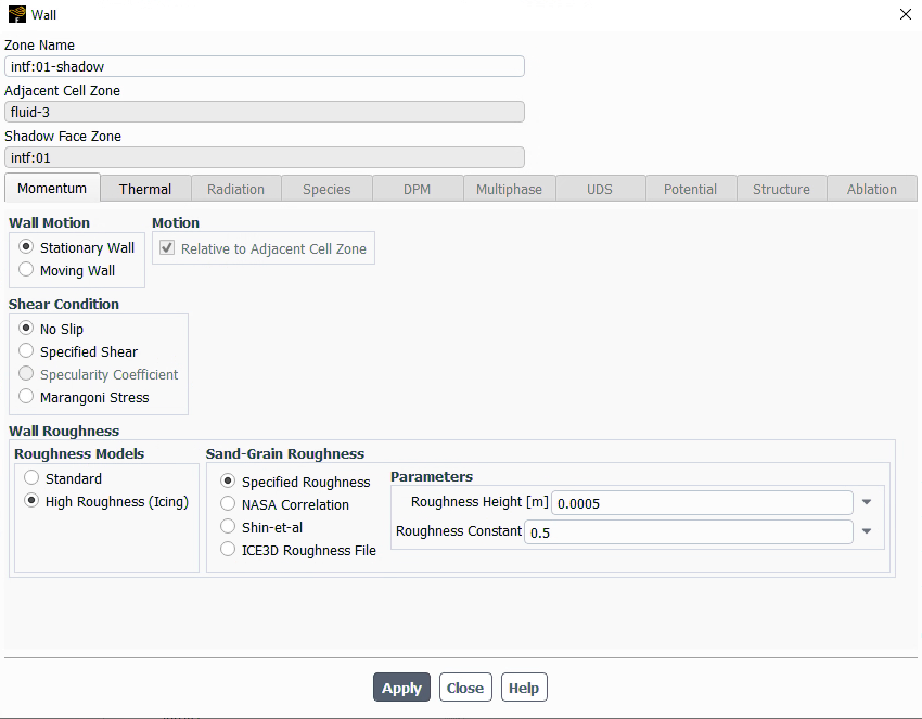
In the Momentum section, retain the following settings:
for Wall Motion.
for Shear Condition.
for Roughness Models.
for Sand-Grain Roughness.
0.0005for Roughness Height [m].0.5for Roughness Constant.
In the Thermal section, retain the following setting:
for Thermal Conditions.
Set the reference values which will be later imported into Fluent Icing.
Setup → Reference
Values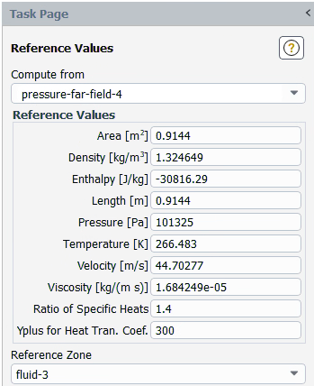
In the Reference Values task page, retain the following setting:
for Compute from.
Setup the solution method.
Solution → Methods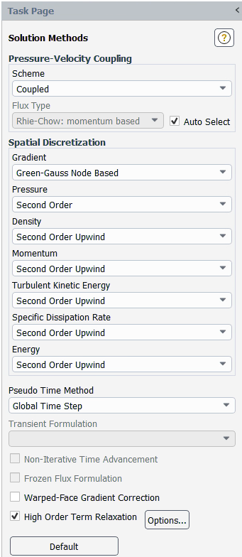
In the Solution Methods task pages, retain the following setting:
for Scheme.
In the Spatial Discretization section, retain the following settings:
for Gradient.
All remaining should be set to either or .
In the Console, type the command below to set the legacy boundary treatment.
/solve/set/nb n
Setup the residual monitors.
Solution → Monitors → Residual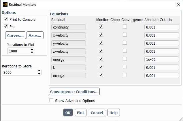
In the Options section, retain the following setting:
Enable and .
In the Equations section, retain the following setting:
Disable all check boxes located under Check Convergence.
Press to close this window.
Setup the initialization method.
Solution → Initialization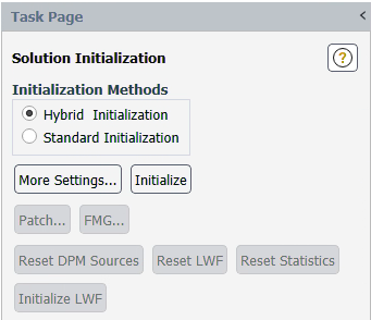
In the Solution Initialization section, retain the following setting:
Hybrid Initialization for Initialization Methods.
Click to initialize the computational domain.
Launch the steady state calculation.
Solution → Run
Calculation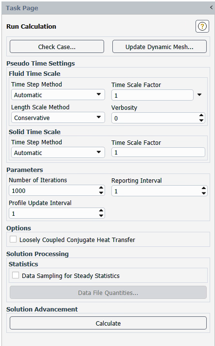
In the Run Calculation section, retain the following setting:
for Time Step Method.
1for Time Scale Factor.for Length Scale Method.
1000for Number of Iterations.
Click to start the calculation.
When the calculation completes, save your solution. Save the solution as deicer_steady.dat.h5 and close Fluent.
File → Write
→ Data...When the unheated steady state CHT solution is verified and ready, the next step is to configure your settings for the initial droplet and icing calculations.
Launch Fluent Icing.
Launch Fluent 2025 R2 on your computer.
Within the Fluent Launcher, set the Capability Level to CFD Enterprise, then select Icing.
Set Solver Processes to
8under Parallel Processing Options.Click Start.
Alternatively, Fluent Icing can be opened using the icing (on Linux) or icing.bat (on Windows) file inside the fluent/bin/ folder.
Create a new project file.
File → New
Project... Enter
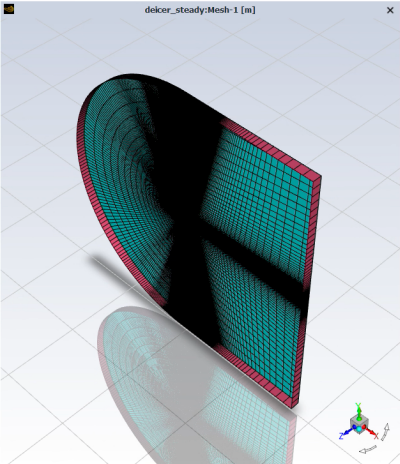
deiceras the Project file name within the Select File dialog.Select and import the deicer_steady.cas.h5 input grid saved in the previous steps.
Project
→ Simulation → Import
Case.A New Simulation window will appear. Enter the Name of the New Simulation as
deicer_transient, and check to enable . Click .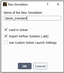
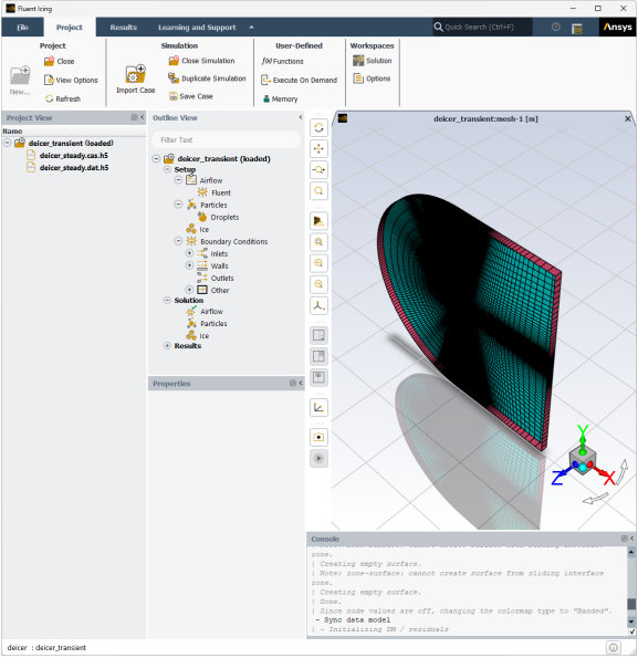
A new simulation folder will be created in the Project View, and the deicer_steady.cas.h5 file will be imported.
After the .cas.h5 file has been successfully loaded, a new Outline View tree appears under deicer_transient (loaded).
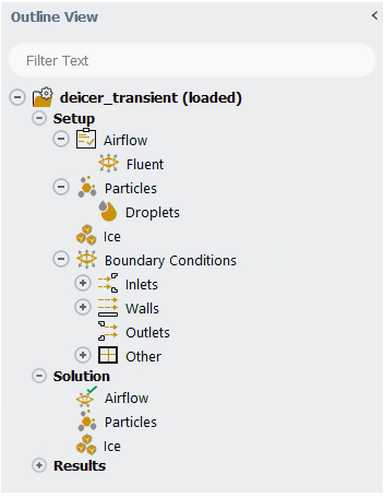
The mesh is now displayed in the Graphics window to the right.
Define the Simulation Type.
Setup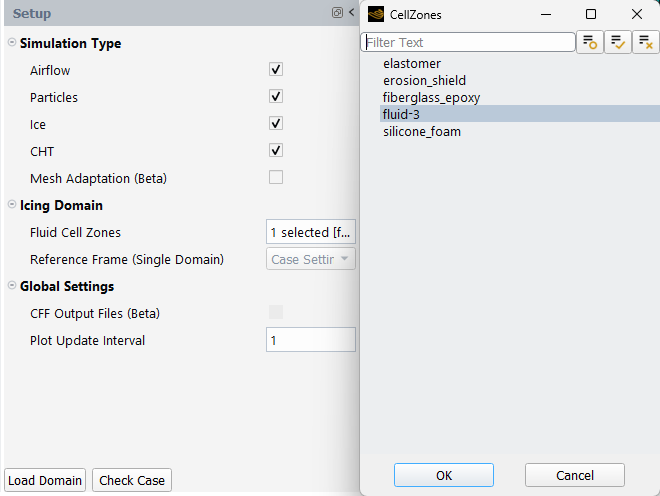
In the Simulation Type section, retain the following setting:
Enable , , and under Simulation Type.
In the Icing Domain section, retain the following setting:
for Fluid Cell Zones.
for Reference Frame (Single Domain)
Click to load the icing domain into icing solver. If a warning message appears, click .
Set the Airflow properties of the simulation.
Setup → Airflow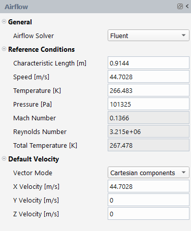
In the General section, retain the following settings:
for Airflow Solver.
In the Reference Conditions section, retain the following settings:
0.9144for Characteristic Length [m].44.7028for Speed [m/s].266.483for Temperature [K].101325for Pressure [Pa].
In the Default Velocity section, retain the following settings:
for Vector Mode.
44.7028for X Velocity [m/s].0for Y Velocity [m/s].0for Z Velocity [m/s].
Set the Fluent properties of the simulation.
Setup → Fluent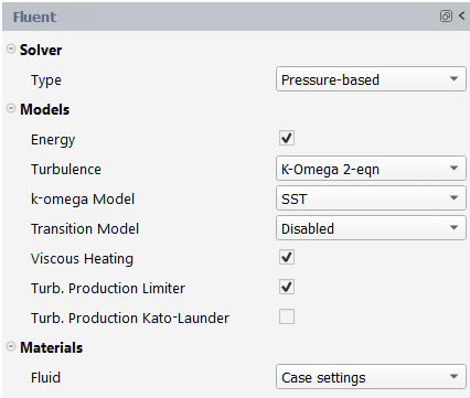
In the Solver section, retain the following setting:
for Type.
In the Models section, retain the following settings:
Enable Energy.
for Turbulence.
for k-omega Model.
for Transition Model.
Enable Viscous Heating.
Enable Turb. Production Limiter.
In the Materials section, retain the following setting:
for Fluid.
Set the Particles properties of the simulation.
Setup → Particles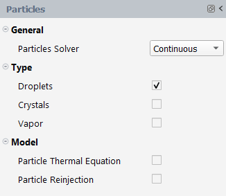
In the General section, retain the following setting:
for Particles Solver.
In the Type section, retain the following setting:
Enable .
Set the Droplets properties of the simulation.
Setup → Particles → Droplets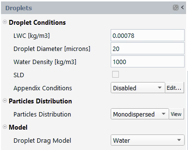
In the Droplet Conditions section, retain the following settings:
0.00078for LWC [kg/m3].20for Droplet Diameter [microns].1000for Water Density [kg/m3].for Appendix Conditions.
In the Particles Distribution section, retain the following setting:
for Particles Distribution.
In the Model section, retain the following setting:
for Droplet Drag Model.
Set the Particles solution properties of the simulation.
Solution → Particles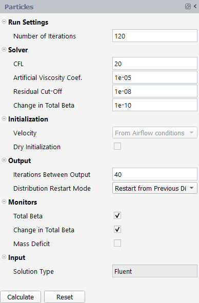
In the Run Settings section, retain the following setting:
120for Number of Iterations.Leave the other settings to their default values.
Run your Particles calculation.
Solution → Particles → CalculateA New run window will appear. Set the Name of the new run to
particles.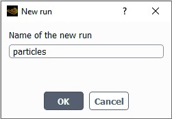
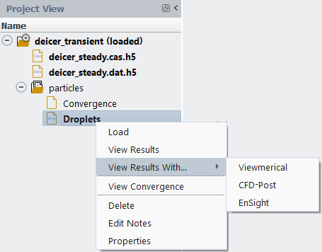
Once particles is complete, view the Droplets solution with Viewmerical. Right-click on the Droplets icon from the Project View and choose → .
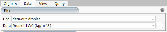
In the Data tab, verify the and on the airfoil. When the droplet solution is verified, move to the next step for the initial icing calculation.
Set the Ice properties of the simulation.
Setup → Ice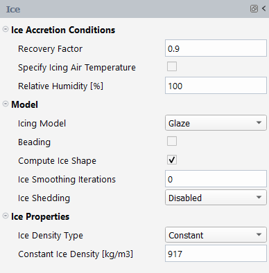
In the Ice Accretion Conditions section, retain the following settings:
0.9for Recovery Factor.Disable Specify Icing Air Temperature.
100for Relative Humidity.
In the Model section, retain the following settings:
for Icing Model.
Disable Beading.
In the Conditions section, retain the following settings:
for Ice Density Type.
917for Constant Ice Density [kg/m3].
Set the Ice solution properties of the simulation.
Solution → Ice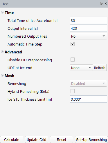
In the Time section, retain the following settings:
30for Total Time of Ice Accretion [s].Enable .
Leave the other settings to their default values.
Run your Ice calculation.
Solution → IceA New run window will appear. Set the Name of the new run to
ice.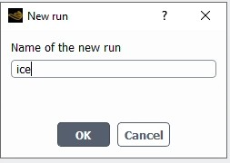
Once ice is complete, view the Ice solution with Viewmerical. Right-click on the Ice icon from the Project View and choose → .
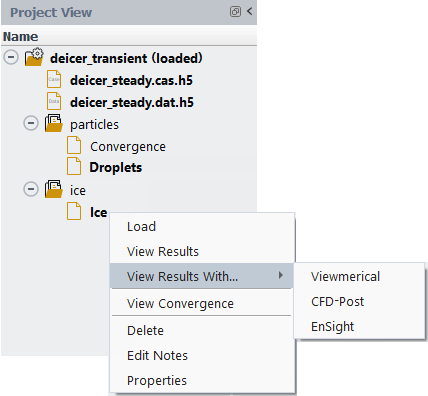
The purpose of the initial ice run is to verify the heat transfer coefficient (HTC) for icing calculation. In Viewmerical, choose the field from the Data dropdown list and verify the CHT distribution. When the ice solution is verified, follow the steps below.
Note: Before running CHT, ensure that the Airflow, Particles, and Ice have completed successfully by displaying green checkmarks on:
Solution → Airflow Solution → Particles Solution → Ice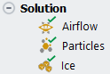
Next, you will set up the de-icing simulation. Unlike anti-icing simulations, de-icing simulations are time-dependent.
Solution → Airflow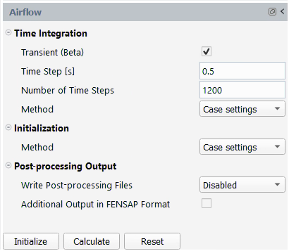
In the Time Integration section, retain the following settings:
Enable .
0.5for Time Step [s].600for Number of Time Steps.for Method.
In the Initialization section, retain the following setting:
for Method.
In the Post-processing Output section, retain the following setting:
for Write Post-processing Files.
The configuration and initial solution are prepared in the Fluent Solution workspaces. Enable it from the ribbon. The Fluent Solution workspace will appear in another window.
Project
→ Workspaces → SolutionCreate the artificial_heater_material material in the Fluent Solution workspace.
Setup → Materials → Solid New...
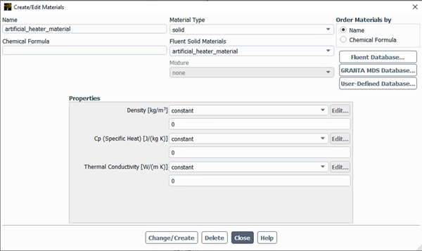
In the Create/Edit Materials dialog box, retain the following settings:
artificial_heater_materialfor Name.Leave Chemical Formula empty.
0for Density [kg/m3].0for Cp (Specific Heat) [J/(kg K)].0for Thermal Conductivity [W/(m K)]. The thermal characteristics are intentionally set to zero.
Press to save your changes.
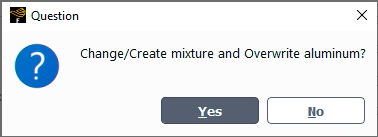
If asked, select to create a new material instead of overwriting the existing one. This material will be used as an artificial material to convert volumetric heat generation rate into surface heat flux.
Press to exit the dialog box.
Define a new expression.
Setup → Named
Expressions New...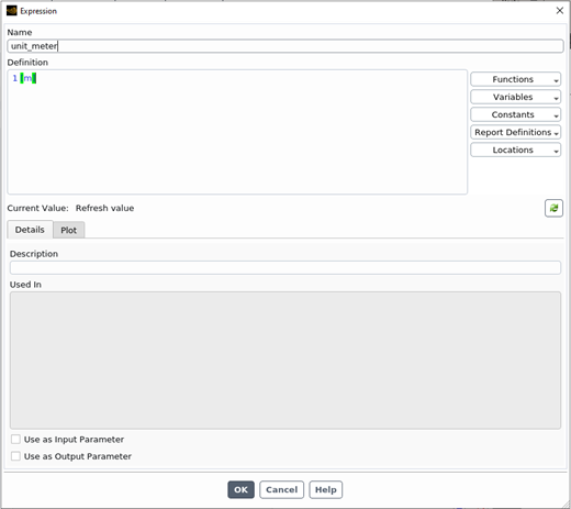
In the Expression dialog box, retain the following settings:
unit_meterfor Name.1 [m]for Defition.Note: If using a different unit system than SI, the length unit must be adjusted accordingly.
Press to continue to the next step.
Define the time-dependent heat power for each heater. The power settings will be entered for 5 cycles.
Setup → Boundary
Conditions WallClick each heater wall boundaries and assign the prescribed heat generation rate shown below.
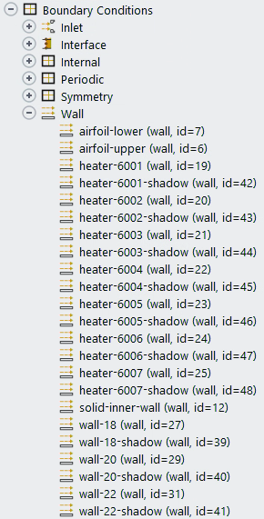
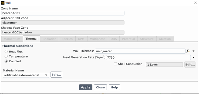
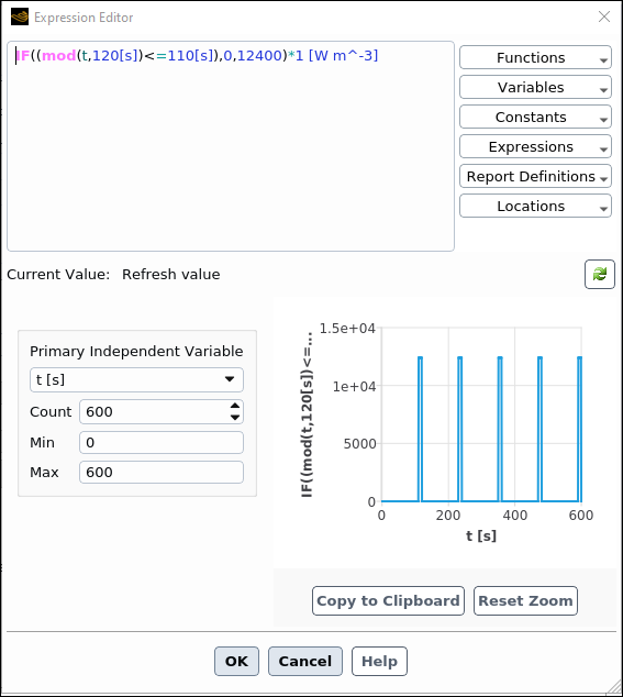
Note: To enter the expression, click the arrow to the right of Heat Generation Rate [W/m3] box and select expression followed the function icon to open the Expression Editor dialog.
Name Heat Generation Rate [W/m3] 6001 77506002, 6003 IF((mod(t+10[s],120[s])<=110[s]),0,15500)*1 [W m^-3]6004, 6005, 6006, 6007 IF((mod(t,120[s])<=110[s]),0,12400)*1 [W m^-3]In the Wall dialog box, for all heaters, retain the following settings:
for Material Name.
unit_meter for Wall Thickness.
Press to continue to the next step.
The de-icing simulation consists of 5 cycles of activation and de-activation of heater pads. Each cycle lasts 120 seconds and has the following properties:
BC Type Start (s) Duration (s) Heat Flux (W/m2) Heater 1 (BC_6001) 0 120 7750 Heater 2 (BC_6002) 100 10 15500 Heater 3 (BC_6003) 100 10 15500 Heater 4 (BC_6004) 110 10 12400 Heater 5 (BC_6005) 110 10 12400 Heater 6 (BC_6006) 110 10 12400 Heater 7 (BC_6007) 110 10 12400 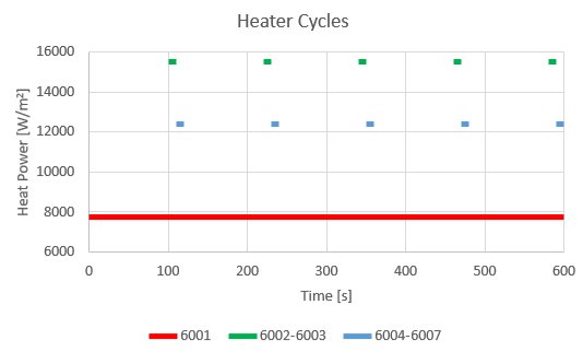
To visualize the expression of the heater power, click on the function. In the Expression Editor, enter the following values:
600for Count.0for Min.600for Max.
Create monitor points to measure the time history of the heaters’ temperature.
Results → Surfaces New
→ Point...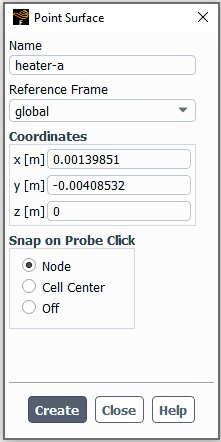
Name Monitor Coordinate heater-a (0.00139851, -0.00408532, 0) heater-b (0.0147708, -0.0186499, 0) heater-d (0.0392124, 0.0296218, 0) surface-probe (0.0245543, 0.0246995, 0) In the Point Surface dialog box, retain the following settings:
heater-afor Name.0.00139851,-0.00408532,0for Coordinates x [m], y [m] and z [m].Repeat the steps above for heater-b, heater-d, and surface-probe using the values found in the table above.
Press to save your changes. Click to proceed.
Create reports for the defined monitors.
Report
Definitions New
→ Surface Report →
Facet Average...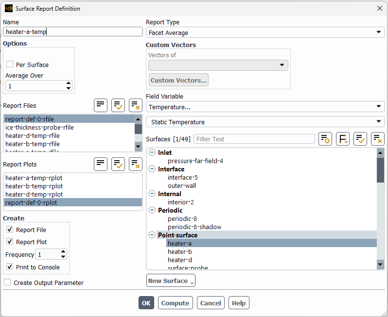
In the Surface Report Definition dialog box, retain the following settings:
heater-a-tempfor Name.for Field Variable.
Repeat the steps above for heater-b and heater-d using the values found in the table above. Name those reports as
heater-b-tempandheater-d-temprespectively.For the ice-thickness-probe, choose and for the Field Variable. This field is available when the initial ice solution is completed and loaded.
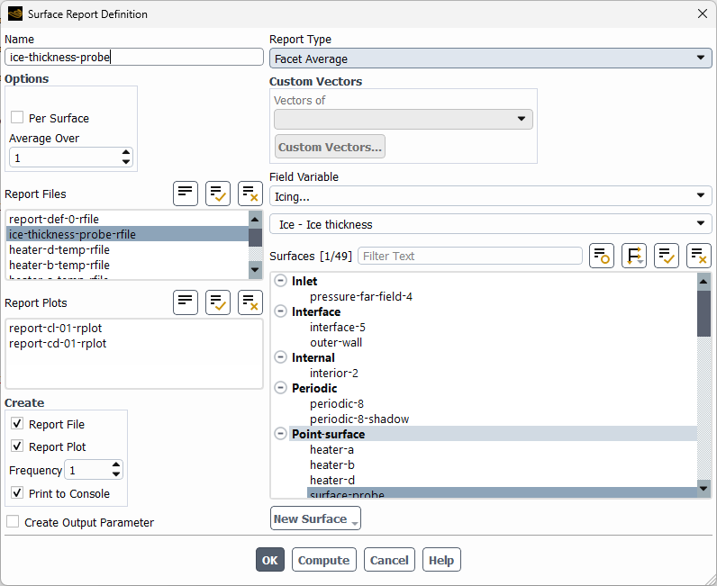
Press to continue to the next step.
The initial solution is critical for the transient calculation. The Patch option can be used to initialize a different solid temperature than the loaded steady state CHT solution.
Solution → Initialization → Patch...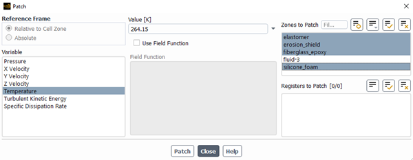
In the Patch dialog box, retain the following settings:
Temperature for Variable.
264.15for Value [K].Select all solid zones (elastometer, erosion_shield, fiberglass_epoxy, silicone_foam).
Press and to exit this window.
The settings on the Fluent Solution workspaces have been completed and the workspace window can be closed.
Project
→ Workspaces → SolutionIn Fluent Icing, set up the CHT de-icing simulation.
Solution → CHT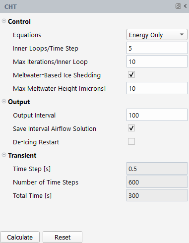
In the Control section, retain the following settings:
for Equations. The thermal coupling between Fluent CHT and icing heat sink will be solved solely using the energy equation. Solving the energy equation alone allows the simulation to run with a relatively larger time step.
5for Inner Loops/Time Step.10for Max Iterations/Inner Loop.Enable .
Keep the default value of 10 microns for the Max Meltwater Height [microns]. The meltwater is typically generated by ice encountered with surface heating from the ice protection system.
The meltwater-based ice shedding model allows ice to detach from the surface if the accumulated meltwater height is above the set criterion. Note that there are several limitations of this model. It assumes that the meltwater does not flow away from its original location. In addition, it does not refreeze into ice even if the surface is cooled below the freezing temperature by any means.
In the Output section, retain the following settings:
100for Output Interval. The solution will be saved at every 10 seconds.Enable .
Note: Saving the intermediate airflow solution is optional but may increase computational time and disk space. However, if a de-icing restart is anticipated, the airflow solution must be saved along with the ice solution to enable a proper and seamless resuming of the calculation.
Disable . Enable this option only for a de-icing restart.
To perform a de-icing restart, enable the option. Right-click both the Airflow and Ice solution that you would like to restart from within the Project View and load them individually. In the example below, the Airflow and Ice restarts are being set to run from loop.05.
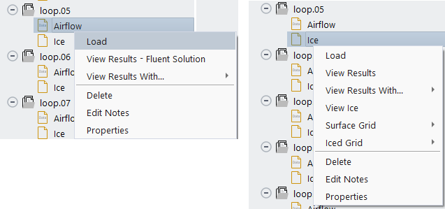
It is good practice to save the case before running your calculation.
Project
→ Simulation → Save
CaseClick to launch the simulation. A New run window will appear. Keep the default name and click to continue. A Convergence window will display the residuals and monitors.
Once your simulation is complete, you can view its convergence graphs in the Graphics window.
Look at the convergence history of the simulation in the Convergence window located on the right of your screen. Set the Dataset to and the Curve to
The time history of the maximum and minimum temperature at the solid interface is plotted. The periodic change of the maximum temperature reflects the cyclic heating of electro-thermal pads. From the Project View, each saved intermediate solution is available and can be viewed by right-clicking the object and selecting and .
Save the case file and close the project.
![]() File → Save
Case
File → Save
Case
![]() File → Close
Project
File → Close
Project