


This section describes the features of the CPU-driven solution mode of Fluent that can be used with the Fluent GPU Solver. The features outlined in this section can be defined after you have read in a previously defined Fluent case file (see Reading Fluent Case Files Into the Fluent GPU Solver) or after reading in a mesh file (see Reading Mesh Files).
This section only covers those settings relevant to setting up your case and does not include information on calculating or postprocessing the GPU solver solution. The settings and procedure for defining calculation activities, calculating the solution, and postprocessing the solution within the Fluent GPU Solver is the same as that of the CPU-driven Fluent solver. Note that the supported features outlined in this section may contain limitations, which are detailed in Fluent GPU Solver Limitations.
Prior to setting up your case in the Fluent GPU Solver, note the following general requirements and capabilities:
The Fluent GPU Solver can only be used with either a single NVIDIA GPU or multiple NVIDIA GPUs with shared/distributed memory. For details on setting specifying GPUs to be used see Starting the Fluent GPU Solver Using the Fluent Launcher or Starting the Fluent GPU Solver from the Command Line.
The Fluent GPU Solver can be used in single precision or double precision.
Multiple CPU processes can be specified for setting up your case and postprocessing the GPU solver solution. See Using CPU Processes for Setup and Postprocessing for details.
Many-to-many CPU/GPU remapping can be used for handling tasks across multiple CPU and GPU resources and can lead to potential performance gains. See CPU/GPU Remapping.
Only 3D geometries are supported.
Mesh topologies with polyhedral, hexahedral, tetrahedral, pyramid, and prism cells, as well as meshes with hanging nodes are supported.
The settings that can be defined when setting up your case within the Fluent GPU Solver are detailed in the following sections:
The following physics modeling capabilities are supported with the Fluent GPU Solver:
Conjugate Heat Transfer (CHT)—including for anisotropic solids—is supported, as described in Specifying the Solid Time Step Size, Time Averaged Explicit Thermal Coupling, and Settings for Anisotropic Solid Zones. Note that the Loosely Coupled CHT option is not supported.
Discrete Ordinates (DO) radiation model as described in Setting Up the DO Model. The DO model is available in combination with the following:
Non-adiabatic FGM (Flamelet Generated Manifolds) combustion model.
Surface-to-Surface (S2S) radiation model. See Setting Up the S2S Model for details.
Species transport with Volumetric reactions or without reactions as outlined in Volumetric Reactions and Species Transport Without Reactions, respectively. Species transport models can be set up with the following settings:
Finite-Rate/No TCI and Eddy-Dissipation turbulence-chemistry interaction models.
Stiff Chemistry Solver and None - Direct Source chemistry solvers.
As described in Partitioning, for simulations with the Laminar, EDC, or PDF transport model, you can partition the mesh in such a way as to promote load balancing. If you enable the Stiff Chemistry option in the Weighting tab of the Partitioning and Load Balancing Dialog Box, you can more evenly distribute the computational load corresponding to the reaction integration.
Flamelet Generated Manifold (FGM) model.
Compressible flows (see Compressible Flows for details).
The following turbulence models are supported:
Laminar
Standard and Realizable k-epsilon
GEKO and k-omega SST
For these models, the Algebraic Transition and Curvature Correction models are supported. For details, see Algebraic Transition Model in the Fluent Theory Guide and Curvature Correction for the Spalart-Allmaras and Two-Equation Models in the Fluent Theory Guide.
For the GEKO model, the Wall Distance Free formulation is supported. For details, see Generalized k-ω (GEKO) Model in the Fluent Theory Guide.
Large Eddy Simulation (LES)
For the LES turbulence model, the following sub-grid scale models are supported:
Smagorinsky-Lilly
WALE
For the LES turbulence model, the following additional model options are available:
Near-Wall-RANS-Layer (WMLES)
When enabled, this option activates the Generic WMLES model (Generic Algebraic WMLES: LES with a Near Wall RANS Layer in the Fluent Theory Guide), which uses LES for the bulk of the domain and the algebraic RANS model for the thin near-wall section of the boundary layer.
Stress-Blended Eddy Simulation (SBES)
Only supported with any of the k-omega models.
Algebraic Transition model. For details, see Algebraic Transition Model in the Fluent Theory Guide.
Curvature Correction model. For details, see Curvature Correction for the Spalart-Allmaras and Two-Equation Models in the Fluent Theory Guide.
Viscous Work is supported for applicable turbulence models. See Including the Viscous Work Effects for details.
For detailed information on setting up the turbulence models listed above see Modeling Turbulence.
Ffowcs Williams & Hawkings acoustics model (see Using the FW-H Model with the Fluent GPU Solver).
Sponge layers acoustics model (see Sponge Layers).
Note that multiple sponge layers are not supported and only one sponge layer can be activated within the Manage Sponge Layers dialog box. If multiple sponge layers are activated, the GPU Solver will only simulate the first sponge layer listed and all other sponge layers will be ignored.
Turbomachinery flows:
Full-wheel and multiple row turbomachinery models.
Transient Rotor-Stator (TRS) with sliding mesh interfaces.
Frozen-Rotor (FR) interface with multiple moving reference frames
Multiple row Periodic Sector simulations, including Periodic Instancing, for both FR and TRS models.
For the Potential model, the following physics modeling capabilities are supported:
Only solid zones are supported
Voltage/current density for wall boundaries:
Time-dependent values are supported.
Contact resistance is not supported.
Coupled boundary conditions
Joule Heating
For the DPM, the following physics modeling capabilities are supported:
Flows and particle treatment:
The DPM is available only for transient particle tracking. However, the model can be used with both steady and transient flow solvers.
When the transient flow solver is used, particles will be injected at the beginning of each flow timestep if the flow time is between the specified injection Start Time and Stop Time. The DPM parcels are created using the CPU Ansys Fluent solver and are then uploaded to the GPU solver. Therefore, DPM parcels cannot be recomputed each time the particle solver is executed. Surface injections with the Randomize Starting Points option enabled will provide random initial positions but these positions will not change each time DPM parcels are injected.
Interaction with the continuous phase:
Both one-way and two-way particle-flow interactions are supported. This is controlled via the Interaction with Continuous Phase option in the Discrete Phase Model dialog box.
In coupled simulations (Interaction with Continuous Phase is enabled), particles can transfer sources into the following flow equations:
Momentum
Energy
Species
The sources are transferred in form of:
mixture fraction sources when the (non)adiabatic FGM combustion model is enabled, and
direct species sources when the detailed species model (that is, the species transport model with volumetric reactions) is enabled.
In coupled simulations (Interaction with Continuous Phase is enabled), you can use the following controls:
DPM Iteration Interval
This allows for tracking particles multiple times within a flow solver time step.
Update DPM Sources Every Flow Iteration
Injection types:
single
group
surface (the face center is randomly distributed over the surface)
file (steady-state only)
cone (all types)
Particle types:
Massless
Inert
Droplet
Injection diameter distribution:
uniform
rosin-rammler
Particle Physical Models:
Note: Most of the physical models for particles are injection-specific.
Drag laws:
spherical
Breakup Model:
SSD
The SSD breakup model is available for spray simulations with droplet breakup due to aerodynamic forces. During droplet breakup, no child droplets will be spawned. Instead, the parent droplet diameter and the number of droplets in the parcel will be adjusted to represent smaller particles while conserving mass. By default, the SSD model uses the following parameter values, which can be adjusted in the Set Injection Properties dialog box (Physical Models tab):
Critical We = 6
Core B1 = 1.73
Xi = -0.1
Target NP = 10
Further physical models:
Convective Heat Transfer
Gravity / Buoyancy
Turbulent dispersion of particles via the discrete-random-walk dispersion model with the Number of Tries fixed at 1, and Time Scale Constant fixed at 0.15.
Evaporation/Boiling:
Evaporation/boiling can be modeled only under the following conditions:
The particle type is Droplet.
Particle material is single-component.
Either the species transport model or nonadiabatic FGM combustion model is enabled.
Only the convection/diffusion-controlled model is available for modeling droplet vaporization.
Switching between evaporation and boiling is based on the particle material vapor pressure.
The Pressure Dependent Boiling and Temperature Dependent Latent Heat options are exclusively used with the GPU solver.
The concept of "DPM Laws" is not available for the DPM with the GPU solver.
The Fluent GPU Solver supports the following material properties:
Density:
piecewise-linear
piecewise-polynomial
polynomial
ideal-gas
incompressible-ideal-gas
boussinesq
constant
Cp:
constant
piecewise-linear
piecewise-polynomial
polynomial
kinetic-theory
mixing-law
Thermal Conductivity:
constant
piecewise-linear
piecewise-polynomial
polynomial
kinetic-theory
cyl-orthotropic
orthotropic
anisotropic
mass-weighted-mixing-law
The cyl-orthotropic, orthotropic, and anisotropic options listed above are available when simulating conjugate heat transfer with anisotropic/orthotropic conductivity for solids. For details see Anisotropic Thermal Conductivity for Solids.
Viscosity:
constant
piecewise-linear
piecewise-polynomial
polynomial
kinetic-theory
sutherland
mass-weighted-mixing-law
Molecular Weight, Standard State Enthalpy, Standard State Entropy, and Reference Temperature:
constant
Mass Diffusivity:
constant dilute approximation
kinetic-theory
Electrical Conductivity:
constant
piecewise-linear
piecewise-polynomial
polynomial
expression
For more details on setting up material properties for your simulation see Physical Properties.
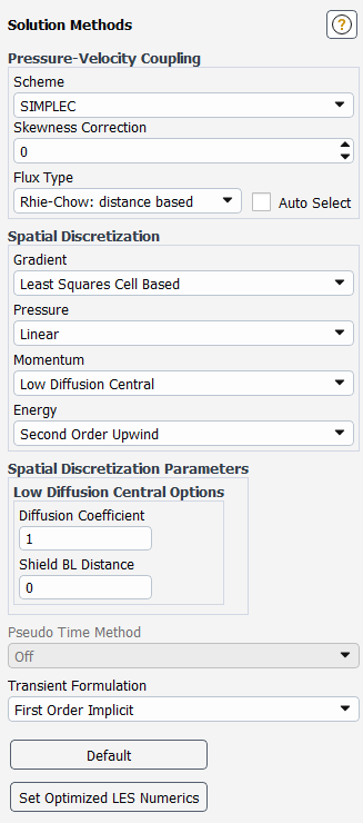
The Fluent GPU solver supports the pressure-based solver with absolute velocity formulation for both transient and steady-state calculations. The following solution methods are supported for the pressure-based solver:
Pressure-velocity coupling can be specified as Coupled (steady state only), or segregated with the SIMPLE and SIMPLEC schemes.
Note: When using the Coupled solver (steady state), both CFL-based and pseudo transient (Global Time Step) time stepping are supported as outlined in CFL-Based Time Stepping and Performing Calculations with a Pseudo Time Method, respectively.
For Flux Type, you can choose either Rhie-Chow: momentum based (default) or Rhie-Chow: distance based (activated automatically for Optimized LES Numerics)
Spatial Discretization
Least Squares Cell Based scheme for gradient.
First-order and second-order discretization schemes for the flow equations.
For pressure, Linear and Body Force Weighted are also available.
The Bounded Central Differencing scheme for momentum and energy is available when the Large Eddy Simulation (LES) or Stress-Blended Eddy Simulation (SBES) turbulence models are enabled.
When enabled, under Spatial Discretization Parameters, you can modify the Bounded Central Diff. Boundedness.
The Low Diffusion Central scheme for momentum is available when the Large Eddy Simulation (LES) or Stress-Blended Eddy Simulation (SBES) turbulence models are enabled.
When enabled, under Spatial Discretization Parameters, you can modify the Diffusion Coefficient and Shield BL Distance.
For incompressible time-dependant calculations, first-order and second-order implicit schemes are supported as well as the Bounded Second Order Implicit scheme for the Transient Formulation (for details see Performing Time-Dependent Calculations).
When the Transient Formulation is set to Second Order Implicit or Bounded Second Order Implicit, the Use limiter in time option becomes available. When enabled, this option will improve boundedness for transient thermal simulations.
When energy is enabled for transient CHT simulations, the Specify Solid Time Step Size option becomes available in the Run Calculation task page for specifying solid-dependent timestepping.
Note: Solid-specific timestepping does not behave the same between the CPU-based and GPU solvers.
When using the Coupled solver, the Flow Courant Number can be specified in the Solution Controls task page when Pseudo Time Method is set to Off.
Set Optimized LES Numerics - When clicked, sets an optimized solution scheme for LES cases. For details, see Optimized LES Numerics .
Both poor mesh numerics and poor mesh removal are supported and can be specified as described below.
Poor mesh removal:
For poor quality meshes containing invalid cells, you can incorporate poor mesh removal by entering the following TUI command, which will delete any cells with left-handed faces:
solve/set/poor-mesh-robustness/poor-mesh-removal/enable?
            Yes
The orthogonal quality threshold is used for marking poor quality cells for poor mesh removal, you can modify the threshold value by entering the following TUI command:
solve/set/poor-mesh-robustness/poor-mesh-removal/orthogonal-quality-threshold
Poor mesh numerics:
The orthogonal quality threshold is used for marking poor quality cells for poor mesh numerics, you can modify the threshold value by entering the following TUI command:
solve/set/poor-mesh-robustness/poor-mesh-numerics/orthogonal-quality-thresholdFor poor quality meshes encountering solver stability issues, you can incorporate poor mesh numerics by entering the following TUI command, which will apply numerics treatments to enhance solver robustness:
solve/set/poor-mesh-robustness/poor-mesh-numerics/enable?
            Yes
For steady-state cases, Data sampling for Steady Statistics is supported within the Run Calculation task page.
For additional information on specifying the above solver settings, see Choosing the Spatial Discretization Scheme.
Note that when using the GPU solver, the following console message can be safely ignored:
Following contexts active in the case file have been de-activated because of their current context
control conditions: "coupled-pseudo-transient"
An optimized LES numerics scheme in available for the GPU solver. The optimized scheme typically allows for a reduction in the number of iterations used per time step (two iterations are often sufficient). In the case of continuity residuals not dropping for the second iteration, reducing the time step size provides better accuracy improvements over increasing the number of iterations per time step used, and eventually leads to better continuity residual behavior.
From the Solution Methods task page, when Large Eddy Simulation (LES) is selected on the Viscous Model dialog box, the Set Optimized LES Numerics button is available at the button of the task page as shown below.
Upon activation, Optimized LES Numerics tunes various details of the discretization and solution algorithm as outlined below:
Underrelaxation Factors
Optimized LES Numerics can typically be run on high quality meshes with high under-relaxation factors (URFs). The default URFs are set to 0.95 for momentum and 1.0 for pressure. For cases with lower mesh quality or when divergence is experienced, lowering the URFs may be necessary.
Using high URFs in combination with the other numerics changes listed below allows the simulation to run using a low iteration count per time step. Iteration numbers are empirical and may differ between cases depending on time step size, mesh quality, and physical models used.
For cases setup with constant density and using Optimized LES Numerics, it is often sufficient to use two iterations per time step without loss of accuracy in results. For cases using ideal gas, five iterations are often sufficient. For cases with poor residual convergence, lowering the time step is usually the better choice in comparison to increasing iteration counts as the computational cost difference may be similar but the results become more accurate.
Low Diffusion Central Advection Operator
Optimized LES numerics uses a low-diffusion central advection operator that is suited
for scale resolving simulations that involve LES. Velocity is reconstructed to cell faces
uses a central scheme. Based on a constant  , and a solution-based smoothness-indicator
  , up-winding is introduced by the jump term of two approximate third
order face velocity reconstructions, each of which has a biased stencil to the respective
side. For a scalar quantity
, up-winding is introduced by the jump term of two approximate third
order face velocity reconstructions, each of which has a biased stencil to the respective
side. For a scalar quantity  , the face reconstruction is
 | (38–1) |
Important: The method does not recover first order upwind even for strong local maxima or minima of velocity and is thus not applicable to capture shocks (that is, not total variation diminishing).
Pressure Scheme
Optimized LES numerics uses a linear reconstruction of pressure to faces when computing the pressure gradient using weights based on cell geometry. This discretization is second order accurate for stretched Cartesian cells and reduces to first order for skewed cells.
Important: The Linear pressure scheme implemented in the GPU solver differs from the CPU implementation. The face pressure still depends on the adjacent cell pressures only, but it is more accurate when the mesh spacing is nonuniform.
Mass Flow Discretization
Optimized LES Numerics uses the Distance-based flux scheme for the face mass flow discretization by default. With this setting, and when the low-diffusion central advection scheme is active, the face mass flow discretization (including Rhie and Chow pressure dissipation) is tuned for accuracy when using LES and low iteration counts per time step.
The following solver settings are available for the DPM:
The particle tracker uses exclusively the High-Res Tracking option. (See High-Resolution Tracking for details.)
Barycentric interpolation is used to interpolate flow solver variables like velocity and turbulence quantities to the particle position. By default, Ansys Fluent will use cell-center values of flow density and viscosity when calculating forces on the particle. If these properties vary with position, it is recommended that they are interpolated to the particle position as well. (See High-Resolution Tracking for details.)
Some of the particle numerical methods cannot be modified:
The trapezoidal Euler scheme is used to calculate the particle position.
The first order implicit Euler scheme is used for particle momentum and energy.
The explicit Euler scheme is used to calculate species and mass.
See Numerics for Tracking of the Particles for more information about these schemes.
The particle integration timestep will be calculated from the Step Length Factor set in the Discrete Phase Model dialog box.
The Accuracy Control tracking option is not available.
In coupled simulations, Linearize Source Terms is available (applied to momentum and energy sources). (See Linearized Source Terms for details.)
The Fluent GPU solver supports updating parametric studies sequentially for variations in supported parameters. For more information on performing a sequential parametric study see Performing Parametric Studies.
This section describes the cell zone and boundary conditions that can be defined when using the Fluent GPU Solver.
The boundary conditions listed below can be defined as constant or as input parameters. Additionally, certain boundary condition settings can also be defined using a steady-state profile, as described in Profiles. Note that input parameters and steady-state profiles are not supported for Mass Flow Rate and Speed for rotational wall motion.
The Fluent GPU Solver supports the following boundary conditions:
Inlet
Velocity-inlet. See Defining the Velocity for details.
Pressure-inlet. See Pressure Inlet Boundary Conditions for details.
Mass-flow-inlet. See Mass-Flow Inlet Boundary Conditions for details.
Intake Fan. See Intake Fan Boundary Conditions for details.
Inlet Vent. See Inlet Vent Boundary Conditions for details.
Outlet
Pressure-outlet. See Pressure Outlet Boundary Conditions for details.
Mass-flow-outlet. See Mass-Flow Outlet Boundary Conditions for details.
Outlet Vent. See Outlet Vent Boundary Conditions for details.
Exhaust Fan. See Exhaust Fan Boundary Conditions for details.
Pressure-far-field
Symmetry. See Symmetry Boundary Conditions for details.
Wall
Stationary Wall and Moving Wall, including Rotational wall motion. See Wall Boundary Conditions for details.
No Slip condition for both stationary and moving walls.
Zero Specified Shear (free slip walls).
Thermal conditions. See Thermal Boundary Conditions at Walls for details.
Wall Thickness thermal condition.
Periodic
Translational. See Periodic Boundary Conditions for details.
Rotational. See Periodic Boundary Conditions for details.
Non-conformal interface boundaries
Fluid-fluid
Fluid-solid
Solid-solid
Rotational and Translational Periodicity
Matching & non-matching interfaces
Porous Jump. See Porous Jump Boundary Conditions for details.
Internal Fan
Single sponge layer at boundary zones.
The following boundary conditions can be defined for both incompressible and compressible flows:
Velocity-inlet
Mass-flow-inlet
Mass-flow-outlet
The following settings can be specified for fluid cell zone conditions:
Frame Motion for Moving reference frames (MRF). See Modeling Flows with Moving Reference Frames for details.
Mesh Motion. See Defining Zone Motion for details.
Porous Zone. See Porous Media Conditions for details.
Source Terms for heat, momentum, and species are supported, as outlined in Defining Mass, Momentum, Energy, and Other Sources, and can be defined as constant or using a steady-state profile.
Reaction mechanisms for species transport with reactions. See Specifying a Reaction Mechanism for details.
3D Fan Zone. See 3D Fan Zones for details.
This section describes the customization options that are available for supported physics models in the context of cell zone and boundary condition setup.
A profile means tabulated data that you supply as a field:
steady profiles are solver‑independent profile data.
transient profiles (beta support) are time varying profile data.
The expressions are of the following types:
parametric expressions depend on design variables that are usually expected as numbers,
Example: 100 [rad/s]
static expressions are expressions that are fully evaluated at the time of initialization,
Example: 1-x^2 - y^2
Note that parametric expressions are a subset of static expressions
Dynamic or time‑dependent expressions are evaluated dynamically as the solver converges,
Example: (1-x^2 - y^2)*VolumeAve(u, ['fluid'])
Example: (1-x^2 - y^2)*sin(t)
Note: Neither expressions nor profiles are supported for setting up models that are not contained in the tables below, such as Species, Combustion, or Radiation. However, there is support for expressions with report definitions and unsteady statistics for Combustion, Momentum, Energy, Viscous, and Electric Potential models. For details about such expressions, see Using Expressions with Report Definitions and Unsteady Statistics.
Table 38.1: Material Cell Zone Conditions
| Zone | Property |
|---|---|
| Fluid |
Density:
|
|
Thermal Conductivity:
| |
|
Viscosity:
| |
|
UDS Diffusivity:
| |
|
Electrical Conductivity:
| |
| Solid |
Density:
|
|
Thermal Conductivity:
| |
|
Electrical Conductivity:
|
Table 38.2: Momentum - Operating Conditions
| Option | Property |
|---|---|
| Gravity |
X Component:
|
|
Y Component:
| |
|
Z Component:
|
Table 38.3: Momentum - Cell Zone Conditions
| Option | Zone | Properties |
|---|---|---|
| Frame Motion | Fluid |
Rotation-Axis Origin:
Rotation-Axis Direction:
Rotational Velocity:
Translational Velocity:
|
| Solid |
Rotation-Axis Origin:
Rotation-Axis Direction:
Rotational Velocity:
Translational Velocity:
| |
| Mesh Motion | All zones |
Rotation-Axis Origin:
Rotation-Axis Direction:
Rotational Velocity:
Translational Velocity:
|
| Source Terms | All zones |
X Momentum:
Y Momentum:
Z Momentum:
|
| Fixed Values | All zones |
X Velocity:
Y Velocity:
Z Velocity:
|
| 3D Fan Zone | All zones |
All properties:
|
| Porous Zone | All zones |
All properties:
|
Table 38.4: Momentum - Boundary Conditions
| Option | Properties |
|---|---|
| Velocity Inlet |
Normal to Boundary
Magnitude and Direction
Components
|
| Pressure Inlet |
Normal to Boundary
Direction Vector:
|
| Pressure Far Field |
Normal to Boundary:
Direction Vector:
|
| Pressure Outlet |
Normal to Boundary:
Direction Vector:
|
| Intake Fan |
Normal to Boundary
Direction Vector:
|
| Exhaust Fan |
Normal to Boundary
Direction Vector:
|
| Inlet Vent |
Normal to Boundary
Direction Vector:
|
| Outlet Vent |
Normal to Boundary
Direction Vector:
|
| Wall |
Moving Wall:
|
Note:
Profile and expression can not be applied simultaneously for one or more of the three velocity components
If transient profile is specified for one component, then the two remaining components must also be specified as transient profile
Axis and Origin must be constant, parametric expression
Table 38.5: Energy Model - Cell Zone Conditions
| Option | Properties |
|---|---|
| Source Terms | Energy:
|
| Fixed Values | Temperature:
|
Table 38.6: Energy Model - Boundary Conditions
| Option | Properties |
|---|---|
| Velocity Inlet | Total Temperature:
|
| Pressure Inlet | Total Temperature:
|
| Pressure Far Field | Total Temperature:
|
| Pressure Outlet | Backflow Total Temperature:
|
| Intake Fan | Total Temperature:
|
| Exhaust Fan | Backflow Total Temperature:
|
| Inlet Vent | Total Temperature:
|
| Outlet Vent | Backflow Total Temperature:
|
| Wall |
Heat Flux:
Wall Thickness:
Heat Generation Rate:
Temperature:
Heat Transfer Coefficient:
Free Stream Temperature:
External Radiation Temperature:
External Emissivity:
|
Table 38.7: Viscous Model - Cell Zone Conditions
| Option | Properties |
|---|---|
| Frame Motion | N/A |
| Mesh Motion | N/A |
| Source Terms | N/A |
| Fixed Values | N/A |
| 3D Fan Zone | N/A |
| Porous Zone | N/A |
Table 38.8: Viscous Model - Boundary Conditions
| Option | Properties |
|---|---|
| Velocity Inlet | Turbulent Kinetic Energy:
|
| Pressure Inlet | Turbulent Kinetic Energy:
|
| Pressure Far Field | Turbulent Kinetic Energy:
|
| Pressure Outlet | N/A |
| Mass Flow Inlet | Turbulent Kinetic Energy:
|
| Mass Flow Outlet | N/A |
| Intake Fan | Turbulent Kinetic Energy:
|
| Exhaust Fan | N/A |
| Inlet Vent | Turbulent Kinetic Energy:
|
| Outlet Vent | N/A |
| Wall | N/A |
Table 38.9: UDS Model - Cell Zone Conditions
| Option | Properties |
|---|---|
| Source Terms | UDS:
|
| Fixed Values | UDS:
|
Table 38.10: UDS Model - Boundary Conditions
| Option | Properties |
|---|---|
| Specified Value | UDS:
|
| Specified Flux | UDS:
|
Table 38.11: Electric Potential Model - Cell Zone Conditions
| Option | Properties |
|---|---|
| Source Terms Potential |
|
Table 38.12: Electric Potential Model - Boundary Conditions
| Option | Properties |
|---|---|
| Potential |
Supported for all boundary conditions:
|
| Current Density |
Supported for all boundary conditions:
|
Table 38.13: VOF Model - Boundary Conditions
| Option | Properties |
|---|---|
| Volume Fraction |
|
The DPM boundary conditions are supported with the following:
inlet
outlet
wall
symmetry
conformal translational or rotational periodic interfaces
nonconformal interfaces with and without translational or rotational periodicity
At inlets, outlets and walls, the supported particle boundary types are “reflect”, “escape”, and “trap”.
For walls that lie within a non-overlap region of a nonconformal interface, only the "reflect" BC type is supported. In this case, you can specify coefficients of restitution for particle reflections for non-overlap regions in the Wall dialog box (DPM tab).
This section describes the solution monitors that are supported by the Fluent GPU Solver.
Note:
When using solution monitors and report definitions, you can increase the solver performance by using the
-gpu_asynccommand line option, as described in Asynchronous Outputting.Solution monitors cannot be created on the following user-defined surfaces:
Iso-surfaces
Iso-clips
Zone surfaces
Quadric-surfaces
The report definitions listed below can be created on an existing surface (boundary condition) or on a Point..., Plane..., or Line... surface. The GPU Solver supports convergence conditions based on the values from report definitions. Additionally, plot, print, and write functionality is supported for both steady and unsteady monitors.
Force
For details on defining the following force reports see Force and Moment Report Definitions.
Drag...
Lift...
Moment...
Force...
Flux
For details on defining the following flux reports see Flux Report Definition.
Mass Flow Rate...
Total Heat Transfer Rate...
Electric Current Rate...
Surface
For details on defining the following surface reports see Surface Report Definitions.
Note: The GPU solver can only correctly report Mass Flow Rate on interior zones, all others are reported as
0values. If you require a surface report definition on another quantity on the interior, try using a plane surface (Plane Surfaces) instead of an interior surface.Area...
Area-Weighted Average...
Facet Average...
Facet Maximum...
Facet Minimum...
Flow Rate...
Integral...
Mass Flow Rate...
Volume Flow Rate...
Mass-Weighted Average...
Sum...
Standard Deviation...
Uniformity Index - Mass Weighted...
Uniformity Index - Area Weighted...
Volume
For details on defining the following volume reports see Volume Report Definitions.
Mass-Average...
Mass Integral...
Mass...
Max...
Min...
Volume...
Volume-Average...
Volume Integral...
Sum...
Expression...
Note: Expression report definitions can only be used on boundary zones and cell zones that exist in the mesh and are used by the solver, as user-defined surfaces and points are not supported.
The following field variables are supported for the above report definitions:
Pressure...
Static Pressure
Dynamic Pressure
Total Pressure
Pressure Coefficient
Density...
Density
Velocity...
Velocity Magnitude
X Velocity
Y Velocity
Z Velocity
Q Criterion Normalized
Lambda 2 Criterion
Temperature...
Static Temperature
Total Temperature
Total Energy
Total Enthalpy
Enthalpy
Turbulence...
TKE (k)
TDR (epsilon)
Turbulent Viscosity
specific-diss-rate(omega)
Materials...
Thermal Conductivity
Laminar Viscosity
CP
Molecular Viscosity
Wall Fluxes...
Wall Adjacent HT Coef.
Wall Shear Stress
Total Surface Heat Flux
Yplus Based Heat Tran. Coef.
Wall Statistics...
Mean Heat Flux
Species...
Mass Fraction
Mean Mixture Fraction
Un-normalized Progress variable
Mixture Fraction Variance
Un-normalized Progress variable variance
Progress variable variance
Progress variable
Radiation...
Incident Radiation
Absorption Coefficient
Scattering Coefficient
Absorbed Radiation Flux
Reflected Radiation Flux
Transmitted Radiation Flux
Absorbed Irradiation Flux
Reflected Irradiation Flux
Transmitted Irradiation Flux
Mesh...
X-Coordinate
Y-Coordinate
Z-Coordinate
Potential...
Electric Potential
Joule Heat Source
dPotential/dx
dPotential/dy
dPotential/dz
The following DPM post-processing capabilities are available:
Mass-in-domain DPM monitor for reporting current particle mass (in kg) or the change rate in mass (in kg/s) in the domain.
Injected-mass, escaped-mass, and evaporated-mass monitors for reporting the mass (in kg) or flow rate (in kg/s) for the given flow solver time step. They differ from the same reports obtained using the CPU solver where the mass is integrated over the tracking period.
Sampling of particle data can be done at face zones and user-defined planes. Sampling on postprocessing surfaces/planes is not supported.
Note that all particles from all injections will be sampled, and the selection of injections in the Release From Injections list in the Sample Trajectories dialog box will be ignored.
Pathlines can be displayed; however, they will be calculated using the CPU solver.
With the GPU solver, you can use expressions with report definitions and unsteady statistics. For details on setting up an expression report definition and unsteady statistics, see Expression Report Definition and Inputs for Time-Dependent Problems, respectively.
The report definitions can be created on an existing surface (boundary condition), and they can be used to generate report files and/or report plots of scalar quantities of interest that you want to monitor during the solution process. When defining the Expression Report Definition dialog box, you can enter the expression directly in the text field, enter the name of a previously created named expression, or use a combination of both. Note that one expression report definition cannot reference another report definition.
The following fields are supported for report definitions and unsteady statistics:
Spatial and Temporal Coordinates
Position: (Cell centroids, Face centroids) (x, y, z)
Time Fields: Time, Flow-Time, Delta-Time
Flow and Thermodynamic Quantities
Density: Density
Pressure: StaticPressure, TotalPressure (incompressible), AbsolutePressure, PressureCoefficient, DynamicPressure
Temperature: StaticTemperature
Velocity Components: Velocity (x, y, z), VelocityMagnitude, Velocity.mag
Energy and Enthalpy: SpecificTotalEnthalpy, SpecificTotalEnergy
Turbulence Modeling and Materials
Basic Turbulence Quantities: TurbulentKineticEnergy (k), TurbulenceDissipationRate, Productionofk
Reaction and Combustion
ProgressVariable, ProgressVariableVariance, UnnormalizedProgressVariable, UnnormalizedProgressVariableVariance
FiniteRateSource, TurbulentFlameSpeedSource
MeanMixtureFraction, MixtureFractionVariance
Electric / Magnetic Fields and Current
ElectricPotential, ElectricPotentialGradients
ElectricalConductivity
XCurrent, YCurrent, ZCurrent, CurrentDensityMagnitude
JouleHeatSource
Note: Some variables are not available on face zones (for example, material fields).
Only the following expression operations and functions are supported for expressions with the GPU solver. All of these mathematical functions take inputs in the form of an expression that evaluates to a real number or a real field and return a real number or real field.
Table 38.14: Operations and Functions
|
Description |
Function |
|---|---|
|
Operators |
|
|
Conditional |
|
|
Hyperbolic |
|
|
Mathematical |
|
|
Reduction |
|
|
Trigonometric |
|
Only the following scientific constants are supported for expressions with the GPU solver.
Table 38.15: Scientific Constants
|
Variable |
Description |
Value |
|---|---|---|
|
|
Pi | 3.14159265358979323846 |
|
|
e (base of the natural logarithm) | 2.71828182845904523536 |
|
|
Gas constant | 8.314472 [J K^-1 mol^-1] |
|
|
Acceleration due to gravity | 9.8066502 [m s^-2] |
The Ansys Fluent GPU Solver is able to export solution data as EnSight DVS files. Such files can then be used for postprocessing using EnSight software. Note the following differences when exporting such files when the data was calculated by the GPU solver compared to that generated by the CPU-based solver (as described in EnSight DVS):
Exporting should be faster.
You cannot export data from the nodes, only the cell centers.
You cannot export data from user-created surfaces.
When exporting during a calculation, only one export definition can be created.
The variable names in the exported file may not be identical to those in a file exported by the CPU-based solver, though the meaning of those variable names should be clear. The affected variable names include those for volume fraction and phase-specific properties, among others.
To export solution data after a steady or transient calculation by the Ansys Fluent GPU Solver, perform one of the following:
Use the File/Export/Solution Data... ribbon tab option to open the Export dialog box, select EnSight DVS from the File Type drop-down list, and make selections from the Cell Zones and/or Surfaces lists, as well as the Quantities list. Then click the button and specify the name of the file in the Select File dialog box that opens.
Use the following text command:
file→export→ensight-dvsEnter responses to the prompts to define the exporting. Note that you can end the entries to the
scalarprompts by enteringq. For example, the following exports a file named "myfile" that contains the x- and y-velocity data from surface 1 and cell zones 3 and 13:file/export/ensight-dvs/ myfile (1) (3 13) x-velocity y-velocity q.
To export solution data during a transient calculation by the Ansys Fluent GPU Solver, perform one of the following prior to running the calculation:
Use the File/Export/During Calculation/Solution Data... ribbon tab option to open the Automatic Export dialog box, select EnSight DVS from the File Type drop-down list, and make selections from the Cell Zones and/or Surfaces lists, as well as the Quantities list. Then make selections from the Export Data Every drop-down lists, enter a File Name, and click the button.
Use the following text command:
file→transient-export→ensight-dvsEnter responses to the prompts to define the exporting. Note that you can end the entries to the
scalarprompts by enteringq. For example, the following creates an export definition "export-1" that will export files every 2 time steps named with "myfile" as the prefix, containing the x- and y-velocity data from surface 1 and cell zones 3 and 13:file/transient-export/ensight-dvs/ myfile (1) (3 13) x-velocity y-velocity q export-1 time-step 2.
Note:
When automatically exporting solution data during a calculation, you can increase the solver performance by using the
-gpu_asynccommand line option, as described in Asynchronous Outputting.As is the case when exporting data generated by the CPU-based solver to the EnSight DVS file type, the following apply when exporting GPU solver data after or during a calculation:
Duplicate surfaces cannot be exported to the EnSight software.
The face zones adjacent to selected cell zones are automatically selected for export, even if they are not specified in the face zone list.
Important: When performing automatic export of solution data (Creating Automatic Export Definitions for Solution Data) to EnSight DVS, ensure you have created all the desired report definitions (Monitoring and Reporting Solution Data) prior to beginning export to EnSight DVS format. Once the solver begins exporting, you cannot create or delete any report definitions, since the EnSight software requires a complete history of residuals and report definition data.