


This option enables the transfer of stresses, strains, history variables, and fiber orientations for certain material models between different meshes with varying numbers of integration points and element types. The following options are available:
| SourceFile = STRING | Define the name and, if needed, the path of the source file, (usually a *.dynain file). |
| TargetFile = STRING | Define the name and, if needed, the path of the target file. This should be an LS-DYNA mesh. |
| MappingResult = STRING |
Define the result filename. The mapping result is written to this newly-generated file. |
|
OrientationFile = HISV Nodes | Define this flag to enable transfer of orientations. This notifies the application that orientation data is stored within history variables (HISV). Alternatively, the orientation can be derived from the element nodes (Nodes). See also the BIAX flag under Mapping Options below. The direction from node #1 to node #2 in the order of input is considered. This method may yield accurate results if the mesh was well-aligned initially. |
| TemperatureFile = STRING | File that contains temperatures on nodes, as *INITIAL TEMPERATURE NODE. |
| ElementSetFile = STRING |
File that contains specific element sets considered for mapping. For example, an element set declaration for additional ICP transformations |
| TTInterpolationFile = STRING | Define the filename for the output of through-thickness interpolation results from the source mesh when performing FE-based averaging and interpolation methods. To actually output this file, you must set the WriteTTInterpolationFile flag (see below). |
| AddEleHISVFile# = STRING | Define the name of a file carrying additional element histories. Multiple files can be defined. The first 10 digits of the string should hold the element ID, the following 10 digits should carry some arbitray value, interpreted as an additional history variable at element level. |
| LookupTable# = STRING |
Filename for lookup tables. Values within a single line must be space-delimited. The Envyo application allows history variable lookup based on these user-defined lookup tables, as described in Equation parser. Following the lookup table command, you must define the columns to be considered for variable lookup. See the example in Equation parser. |
| TransformedMeshFile = STRING |
Specify the output filename for the transformed mesh. This option is intended solely for postprocessing of the transformation. For additional details, refer to the Transformation Options section below. |
Available source and result file formats are listed below:
|
SourceFileFormat = LS-DYNA ESI-PC Nastran HDF5 ESI-HDF5 GCODE ABAQUS STEP CSV | The source file format. The preferred format is LS-DYNA. |
|
TargetFileFormat = LS-DYNA ESI-PC | The target file format. The preferred format is LS-DYNA. |
|
ResultFileFormat = LS-DYNA |
The result file format. The only format available is LS-DYNA. |
| NumTargetPIDs = INT | Define the number of parts in the target mesh that are considered within the mapping. This option should be followed by TargetPID#i definitions. |
| TargetPID#i = INT | Define as many part IDs as specified in NumTargetPIDs. These parts are considered for the mapping. |
| NumSourcePIDs = INT | Define the number of parts in the source mesh that are considered within the mapping. This option should be followed by SourcePID#i definitions. |
| SourcePID#i = INT | Define as many part IDs as specified in NumSourcePIDs. These parts are considered for the mapping. |
Note: The options above specifically narrow down the scope of the mapping procedure to defined part IDs. Other parts are ignored on both the source and target meshes.
|
TRANSFORMATION = YES NO |
Enable/disable transformation option. |
|
WriteTransformedMesh = YES NO | Flag to enable output of the transformed mesh used for mapping. This enables success verification for the transformation. If set to YES, a TransformedMeshFile must be specified (see above). |
|
WriteTTInterpolationFile = YES NO |
Activate the output of the through-thickness interpolation result when performing FE-based averaging and interpolation methods for differing source and target through-thickness interpolation rules. The file name is defined with TTInterpolationFile - see Input and Output Meshes above. |
There are three available methods for performing mesh transformation:
TRAFO_OPTION is not required:
User-defined translation and rotation
The 4PCS method should be used with caution, as it is fully automatic and may not accurately transform stress tensors and fiber orientations between different coordinate systems. The ICP algorithm is the recommended approach.
The user-defined translation and rotation options are listed beneath TRAFO_OPTION.
Note: Transformation options are used to transform the source mesh.
|
TRAFO_OPTION = 4PCS ICP | Flag that enables specification of the desired transformation option. |
| NodalPair#i = INT INT |
Define nodal pairs to initialize mesh alignment for the ICP algorithm. You can specify up to ten nodal pairs, with a minimum of three required. In each pair, the first integer represents a node ID in the source mesh, and the second corresponds to a node ID in the target mesh. Input values should be space-separated, with each nodal pair provided on a separate line. |
| Additional Transformations = INT | Define the number of additional transformations conducted using the ICP algorithm. |
| AddTrafo#i = INT | Define as many additional transformation IDs as specified in Additional Transformations. The supplied value represents the element set ID that should be used. |
| AddNodalPair#i = INT INT | Define 4 nodal pairs for additional mesh alignment for the ICP algorithm. |
| MAX_NUM_ITER = INT | Maximum number of iterations to be performed by the 4PCS algorithm. |
| GLOBAL_ERR = DOUBLE | Global error measurement to accept transformation as best fit for the 4PCS algorithm. |
|
MATCHING_POINT_DIST = DOUBLE |
Maximum distance between points such that they are accepted as matching (4PCS). |
|
PERCENTAGE_OF_MATCHING_POINTS = DOUBLE | Percentage of matching points for transformation acceptance (4PCS). |
Additionally, a custom sequence of user-defined transformations can be applied. These transformations are executed in the order in which they are specified and multiple transformations may be defined.
|
RotateSRC = DOUBLE;X DOUBLE;Y DOUBLE;Z DOUBLE; DOUBLE DOUBLE DOUBLE | The source mesh is rotated by a specified angle (first value, in degrees) around a defined axis. Predefined axes are X, Y, and Z. Alternatively, a custom axis can be specified by providing three space-separated floating-point values following a semicolon (; x y z). |
| MoveSRC = DOUBLE DOUBLE DOUBLE | The source mesh is moved along the user-defined vector (x y z). |
| ScaleSRC = DOUBLE | The source mesh is scaled around the origin using the defined scale factor. |
In addition to the transformation options, you can convert the unit systems:
|
ChangeUnitSystem = YES NO | Activate or deactive unit system conversion. |
|
SourceUnitSystem = kg - m - s ton - mm - s kg - mm - ms g - mm - ms lb - in - s | If unit system conversion is activated, provide information about the source unit system. |
|
TargetUnitSystem = kg - m - s ton - mm - s kg - mm - ms g - mm - ms lb - in - s | If unit system conversion is activated, provide information about the target unit system. |
|
ALGORITHM = ClosestPoint ElementSizeSearchRadius ConsiderOndulation RVE_Detection | See descriptions below. |
ClosestPoint is the most commonly-used option and accounts for most of the mapping scenarios targeted by the Envyo application. Beginning with the target mesh, the next element or integration point is identified and its data transferred to the target mesh.
The ElementSizeSearchRadius option supports mapping of results from mesoscale process simulations using shell elements onto a target mesh. The target mesh element size is therefore used as a search radius, whereas the source mesh elements are projected onto the target mesh along the source-mesh normal and a check is performed to see if the intersection is within the target element. The element size can be scaled using Scale_SearchRadius (below).
The ConsiderOndulation option considers the through-thickness position of the identified fiber orientation. This information is therefore not considered as provided by user input, but by the position in the source mesh related to the target mesh. This option does not account for the ordering of the input parts - it first maps those that are closest to the target part, then the second closest and so on. No resinuous areas can be assigned with this option. If the MapThickness option (below) is enabled, the offset between the source layers is also considered, which usually leads to varying thicknesses throughout the part.
With RVE Detection, you can define specific criteria which allows the Envyo application to decide if a specific combination of fibers has been identified and therefore assigns a specific, user-defined material ID to the dedicated integration point.
|
MapStress = YES/NO CP AVG SHEPARD NO1 SHEPARD NO2 SHEPARD NO3 SHEPARD NO4 FE FE NODAL AVG | YES/NO activates/deactivates the mapping of stress data (every value stored in the *INITIAL STRESS OPTION fields on the source side). The default algorithm used is the closest point (CP) algorithm (or nearest neighbour search). For explanations of the other options, see below. |
CP - directly activates the closest point algorithm to transfer everything stored in the *INITIAL STRESS OPTION fields on the source side. This is the default algorithm.
AVG - the euclidean average is taken from the values found within a specific search radius. By default, the search radius is based on the average target mesh element length.
SHEPARD NO1 - activates the general Shepard's inverse distance weighting function. You may specify the exponent using the SHEPARD EXPONENT option.
SHEPARD NO2 - activates the Shepard's inverse distance weighting function, with a minimum of four and a maximum of ten points considered for the interpolation function. You may also specify the exponent using the SHEPARD EXPONENT option.
SHEPARD NO3 - activates the Shepard's inverse distance weighting function, with a minimum of four and a maximum of ten points considered for the interpolation function, including direction. You may also specify the exponent using the SHEPARD EXPONENT option.
SHEPARD NO4 - activates the Shepard's inverse distance weighting function, with a minimum of four and a maximum of ten points considered for the interpolation function, including direction and the slope. You may also specify the exponent using the SHEPARD EXPONENT option.
The search radius for the four options listed above is adjusted based on Shepard's proposal, see [22].
FE - activates the interpolation of values found in the *INITIAL STRESS OPTION fields based on finite element shape functions and point projection of the considered integration points into the plane of the source shells. If the source and target through-thickness integration rules are different, through-thickness interpolation is performed based on the method proposed in [24], minimizing the difference in the areas underneath the through-thickness integration rules on source- and target side for all values being transferred. This interpolation result can be visualized using the WriteTTInterpolationFile and TTInterpolationFile options.
FE NODAL AVG - activates the interpolation of values found in the *INITIAL STRESS OPTION fields based on finite element shape functions and point projection of the considered integration points into the plane of the source shells. In addition to the described method above, values of the connected elements on the source side are also considered through extrapolation of the integration point values onto the element nodes, taking the euclidean average and performing a value recovery on the target integration point.
|
MapStrain = YES NO | Specify whether or not strains should be transferred. |
|
MapThickness = YES/NO CP AVG SHEPARD NO1 SHEPARD NO2 SHEPARD NO3 SHEPARD NO4 FE FE NODAL AVG |
Activate or deactivate thickness transfer. This option requires *ELEMENT SHELL THICKNESS fields in the *.dynain file. If TargetThickness is also defined, it will be ignored. The default option is CP (closest point). Thickness mapping is based on the thicknesses stored on the nodes. Thickness is averaged over all elements attached to a node, regardless of the chosen interpolation option. The listed interpolation options work in a similar way as those described under MapStress. |
|
Thck_Avg_Opt = Ele Avg Nodal Avg |
Thickness averaging option. When using *ELEMENT SHELL THICKNESS, nodes may hold different thickness information, depending on the element to which they belong. This is especially criticial for components with ribs. With the default setting (Ele Avg), the Envyo application calculates through-thickness integration points using the nodal thicknesses stored on the element nodes by interpolating the resulting thicknesses at the in-plane integration points via shape functions, allowing for the correct calculation of the local through-thickness integration points. By choosing the Nodal Avg option, the application first collects all thicknesses stored on one node from its attached elements and averages these thicknesses. Interpolation to the in-plane integration points using shape functions is then performed. |
|
TENSORIALINT = AVG INV-N INV-R INV-K INV-U INV-C | This option controls how tensorial values are interpolated. Only stress tensors are considered with the proposed methods. As these methods are still under development, you should use the default AVG method. |
Besides using the standard euclidean average (AVG), which is the default and recommended value, further interpolation methods based on tensor invariants have been investigated due to the fact that swelling effects are often seen when performing standard euclidean average of tensorial data (the tensor shape changes).
Based on the work of [9], several invariant sets have been implemented for the interpolation functions available in MapStress, and linear interpolation is performed for these invariant sets instead of the single tensorial values. These interpolated invariants allow you to recover the eigenvalues based on a closed form solution of the cubic function and together with the eigenvectors determined through linear interpolation of the originating tensors, the resulting tensor can be recovered.
Due to the boundaries of the recovery function, which is based on the arccosine defined between -1.0 ≤ x ≤ 1.0, this might lead to unexpected behavior with the current implementation.
INV-K refers to an orthogonal invariant set based the tensor trace, the Frobenius norm of the tensor's deviatoric (fractional anisotropy of the tensor), and the mode of the deviatoric.
INV-R refers to an orthogonal invariant set based the tensor norm, the relative anisotropy of the tensor, and the mode of the deviatoric as in INV-K.
INV-N is a non-orthogonal invariant set based on the tensor trace, the fractional anisotropy, and the tensor mode.
INV-U is a uniform invariant set based on the tensor trace, the scaled relative anisotropy of the tensor, and the scaled angular mode AM.
These invariant sets have been proposed in [9] for positive definite tensors gained in DT-MRI measurements. Generally, stress tensors are not positive definite. The Cauchy stress tensor invariant set INV-C is therefore added to the interpolation options, even though this might not solve the issue regarding the arccos in the recovery function.
| TargetThickness = DOUBLE | Define the thickness of the target shell mesh. |
| SHEPARD EXPONENT = DOUBLE |
Define the exponent of the Shepard's inverse distance weighting function. Default = 2.0. |
For cases where the target mesh does not contain any information regarding the integration rules being used, such as element formulation and through-thickness integration points, you must define these manually. The input for this is as follows:
| NPLANE = INT |
1 - reduced integrated thick shell elements 4 - fully integrated thick shell elements This option was formerly known as NumberOfTARInPlaneIPs. |
| NTHICK = INT |
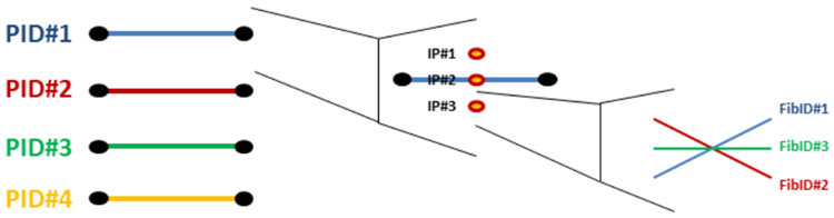
Define the number of through-thickness integration points (IPs). If the Algorithm=RVE Detection option is used, ensure that the number of through-thickness IPs refers to the number of fibers being mapped, the number of source shell element stacks, and the number of through-thickness IPs in the source mesh. The number of through thickness IPs can be reduced using the ThroughThicknessAveraging option (see Further Options ). See also Figure 4.3: Number of stacks, integration points and fiber IDs for *MAT 249 and Note 1 under Notes. This option was formerly known as NumberOfTARThroughThicknessIPs. |
|
IntegrationRule = Gauss Lobatto Autoform Moldflow | Define the through-thickness integration rule for the mapping result. This option directly affects the positions of the through-thickness integration points on the target mesh. |
|
BIAX = YES NO |
If fiber orientation is derived from node numbering, usually only the direction from node #1 to node #2 is used. The BIAX flag activates the additional usage of node #1 to node #4 in order to consider two-directional materials (for example, woven materials). The directions are written to two integration points in the same order as described above. |
| INN = INT | This flag is similar to the invariant node numbering flag in LS-DYNA provided in the /CONTROL ACCURACY field, see [19]. To properly calculate orientations with respect to the element coordinate system, the Envyo application requires information about how LS-DYNA calculates the element coordinate system. The default, as with the LS-DYNA application, is off (0). |
|
Search_Radius = SrcEleLen TarEleLen DOUBLE | The search radius declaration for the mapping algorithm. SrcEleLen is the default, which uses average source mesh element size as the search radius. Average target mesh element size can be used by defining TarEleLen, or a positive DOUBLE value can be defined. |
| Scale_SearchRadius = DOUBLE | Coefficient to scale search radius. For the ElementSizeSearchRadius option, the search radius for element projection is scaled with this factor. The default value is 1.0, meaning that the original element size is used as a search radius. |
| Shell_Option = Composite Composite Long |
This option tells the Envyo application to generate *ELEMENT SHELL COMPOSITE( LONG) elements from the mapped orientations. |
| SORT = BUCKET | Using bucket sort is strongly recommended, as it provides a substantial performance improvement for the search algorithm. |
| REPEAT = YES | Enable this option to ensure that all elements and integration points receive mapped data. When there is a significant difference in element sizes between the source and target meshes, the default bucket refinement may be insufficient to cover all points, sometimes by design. In such cases, this flag must be set to guarantee complete data coverage. |
For the RVE DETECT algorithm, specific properties for representative volume elements must be defined:
| Num_RVEs = INT |
The number of representative volume elements to be searched for through the thickness. |
| RVE# = INT INT;INT |
Using this option, you can specify up to three part-IDs to define a specific RVE, allowing triaxially-braided representative volume elements to be defined. If only biaxial braids or woven materials are available, omit the final integer value. The final integer is interpreted as the reinforcing yarn, whereas the first two integers are considered as rotating yarns for braided composites. The reinforcing yarn should be seperated from the rotating yarns by a semi-colon. |
| RVE_TYPE = BRAID |
Only braided or woven materials can be detected by the algorithm. |
| UD INT |
Define the material ID which should be assigned in cases where only one fiber ID is found within the search radius. |
| BIAX_i INT |
Define the material ID which should be assigned in cases where two fiber directions are found. The index i in BIAX_i points to a specific angle between the two fiber IDs. If several biaxial RVEs are defined, the material ID which points to the closest angle between the two fibers found in the RVE is assigned. The orientation projected onto the target mesh is derived as the average between the two rotating yarns. |
| TRIAX_i INT |
Define the material ID which should be assigned in cases where three fiber directions are found. The index i in TRIAX_i points towards a specific angle between the two rotating yarn fiber IDs. If several biaxial RVEs are defined, the material ID which points to the closest angle between the two rotating yarn fibers found in the RVE is assigned. The direction used for projecting onto the element is derived from the reinforcing yarn direction. |
| FIBER_PRECENTAGE = DOUBLE |
The mininum percentage of fibers which should be considered for the mapping. The Envyo application counts the overall number of fibers found within a specific search radius and checks if the ratio of each fiber is higher than the value specified here. |
| ResinMatID = INT |
This parameter can be set for the ElementSizeSearchRadius option and assignes a specific material ID to integration points where no neighbouring element to assign a fiber orientation could be found. If no value is given, a default is used to assign a material ID for specific resinuous areas. |
Further options for the mapping of fiber orientations from *MAT 249 (*MAT REINFORCED THERMOPLASTIC) [20] are as follows:
| NumFibers = INT |
Define the number of fibers which are stored in *MAT 249 and are considered for the mapping process. |
| FiberID#i = INT |
Define as many fiber IDs as specified in NumFibers. These fibers are considered for the mapping. |
| CMPFLG = 0 | Flag for the output coordinate system for shells, solids and thick shells. Also see *DATABASE EXTENT BINARY in [19]. |
| SourceMaterialModel = INT | Number of the material model used for the generation of the *.dynain file. The only available material model is *MAT 249. |
| POSTV = INT |
Defines the data written to the *.dynain file. POSTV = 63 and POSTV = 8 are supported. As an alternative, you can either define POSTV = 0 or completely ignore this flag. History variables are then expected to be written as default. If the source mesh is generated by LS-DYNA version R9, POSTV = -9 can be defined. Further options will be added on request. |
| TargetMaterialModel = INT | Number of the target material model to which specification the fiber directions should be output. The only available material model is *MAT 249. |
| IHIS = INT | IHIS option for *MAT 249. The only supported option is 1. |
|
ThroughThicknessAveraging = YES NO |
Set to YES (recommended), if orientation averaging is to be performed through the thickness of the source parts, or if a specific stacking sequence is needed to define the fiber orientation. You should use this option in cases where orientations are being transformed and should therefore appear in a specific order, rather than using arbitrary orientations throughout the thickness. If the target material model is defined as *MAT 249, fiber averaging differs slightly. Refer to the respective explanations below. When set to YES, the NumberOfFiberBundles option (below) must be defined. |
| NumberOfFiberBundles = INT | Define how many averaging options should be performed. |
| FiberBundle#i: | Counter for fiber bundles. |
| MatID = INT | Material ID of the fiber bundle. |
| Lay = INT,IP = INT,Fib = INT |
Repeat this field as many times as necessary for each of the averaging possibilities: Lay refers to the Layer (using the same numbering as in SourcePID#i) of stacked elements in the source mesh. IP is the respective IP in that layer. Fib is the respective fiber. All values listed here are averaged until the next different input parameter is defined. |
The Lay=INT, IP=INT, Fib=INT definition should be handled differently for the *MAT 249 target material model. Since this material model can represent up to 3 distinct fiber directions, the direction averaging per target through the thickness integration point should also support up to 3 fiber directions.
The integer value for Fib is considered as a digit-wise value only if target material model is *MAT 249.
This digit-wise integer represented by,


As can be seen above, the digit position represents the store-position on the target mesh and the value represents which source fiber should be used to do averaging. An example is given in note 2.
| InitialStress = DOUBLE | Allows initialization of a specific stress value for all elements and integration points. This flag is mainly used to remove all stresses after mapping is performed, so that InitialStress = 0.0. |
HISV_HANDLING = YES NO CLEAR |
Allows you to move and modify history variables manually. Regarding the meaning of histories, refer to [20], [4]. If CLEAR, all history variables will be removed before generating the result file. If set to YES, define as many history variables as should be modified (see Equation parser). |
| MAX_NUM_HISV = INT | Define the new maximum number of history variables. This is an easy way to get rid of unwanted histories which are of no use for the new model, but also allows you to extend the amount of histories being output. If a history variable is moved to a position which is higher then the actual number of history variables in the input deck, the number of histories is extended automatically. |
An equation parser has been implemented in the Envyo applkication, based on the Shunting yard algorithm and is available as an MIT license [6]. This equation parser has been modified to work with common LSDYNA variables such as histories and effective plastic strains and stresses. Variables are declared using the & symbol and commands are executed in the order of input.
The following variables are supported:
| &HISV#i | History variable at position i. |
| &EPS | Effective plastic strain (the last entry in *INITIAL STRESS SHELL which may have a different meaning than eff. plas. strain). |
| &ELELENGTH | The element length of the current element. |
| &SIG_IJ | Components of the 2nd order stress tensor. |
| &SIG_INIT | Allows initialization of a specific stress value. Refers to all stress components. |
| &ADD ELE HISV#i | Element history variable from file i is used. |
| &LookupTable#i | Lookup table from file i is used. |
| exp | Exponent. An alternative input would be e**. |
The example below illustrates the usage of the equation parser in combination with lookup tables. The commands following the additional history and lookup table definition are executed in the order of input:
Example: History variable manipulation
AddEleHISVFile#1 = Results A.dyn
AddEleHISVFile#2 = Results B.dyn
LookupTable#1 = data A.txt,&COL#1,&COL#2,&COL#3
LookupTable#2 = data B.txt,&COL#1,&COL#2,&COL#3
&HISV#3 = &ADDELE HISV#2
&HISV#2 = &ADDELE HISV#1
&HISV#4 = abs(&HISV#3-&HISV#2)*0.000467354
&EPS = &LookupTable#1,linearInterpolation,&HISV#4,&ELELENGTH,&COL#3
&HISV#6 = &LookupTable#2,nextNeighbour,&EPS,&ELELENGTH,&COL#3
&HISV#8 = &HISV#2
&HISV#9 = &ELELENGTH
MAX_NUM_HISV = 8
Two additional element history files are loaded into the Envyo application and are stored internally. In addition, two lookup table files are read. For each of these, column one, two, and three are considered. These numbers can be different and it is also possible to have more than just three columns.
After reading the data, the following commands are executed:
Additional element history variable from file 2 are stored as history variable # 3.
Additional element history variable from file 1 are stored as history variable # 2.
The value of history variable # 4 are calculated using the absolute value of history #3 - # 2, multiplied by a scale factor.
To get information about the effective plastic strain, lookup table # 1 is used. Linear interpolation is used if values are between two values provided within one of the columns. In this case, history variable #4 is compared to values stored in column # 1.
The application takes the element length of each element and compares it with the values stored in column # 2 of lookup table # 1. The final result is the value provided in column # 3.
The value of history variable # 6 is derived in a similar way, considering the next neighbour instead of performing a linear interpolation between the values. The first input is the resulting effective plastic strain from the previous step. Again, results are provided in column # 3.
Following these operations, history variable # 8 is assigned the value at history variable # 2, and the element length is stored at history variable # 9.
Nevertheless, only eight history variables are written to the final result file due to MAX_NUM_HISV.
Part clustering is available on arbitrary history variables or even stress values. The input is as follows:
CLUSTERID#i = STRING, STRING, DOUBLE, DOUBLE, INT (,INT)
The value at i refers to the old part ID in the target mesh.
The first STRING refers to the history variable or stress component used for part clustering (see Equation parser).
The second STRING refers to the clustering method. Possible inputs are AVG for average or MinMax. In either case, the average of the values stored on integration points is taken for evaluation.
The DOUBLE values refer to the values to which the averaged component (first STRING) is compared. If AVG is selected, these are the exact intervals which are used for comparison. If the MinMax option is chosen, these values are the overall range of history variable values which are split into equaly spaced intervals by the provided optional (last) INT value. The first DOUBLE value refers to .GE., the second DOUBLE value to .LT..
The following INT value refers to the assigned part ID after clustering. If the MinMax option is chosen, this is the starting part ID for the lowest equally spaced range.
The last INT value is only needed for the MinMax option and defines the number of equally spaced splits to be performed.
Example: Clustering
CLUSTERID#500004 = &HISV3,MinMax,1.248,9.120E+02,12,6
Target part ID 500004 is split based on history variable # 3. The MinMax option is chosen, so the application creates 6 equally spaced regions between 1.248 and 9.12E+02. Averaged values of history variable #3 are assigned part IDs starting at part ID 12.
CLUSTERID#500004 = &HISV3,AVG,1.248,2.803E+02,12
CLUSTERID#500004 = &HISV3,AVG,2.803E+02,4.067E+02,13
CLUSTERID#500004 = &HISV3,AVG,4.067E+02,5.330E+02,14
CLUSTERID#500004 = &HISV3,AVG,5.330E+02,6.593E+02,15
CLUSTERID#500004 = &HISV3,AVG,6.593E+02,8.857E+02,16
CLUSTERID#500004 = &HISV3,AVG,8.857E+02,9.120E+02,17
Target part ID 500004 is split based on the average values on each element of history varibale # 3. Averaged values within a range of 1.248 ≤ x < 2.803E + 02 are assigned the new part ID 12, values within the range of 2.803E + 02 ≤ x < 4.067E + 02 are assigned the new part ID 13, and so on.
Note 1:
As shown in Figure 4.3: Number of stacks, integration points and fiber IDs for *MAT 249, *MAT 249 outputs several fibers at each integration point. This must be considered in NTHICK or in the respective averaging options. In the example below, the source file consists of four stacked shell elements (Part 1 - 4), with three integration points through the thickness each, having three fibers each. A complete mapping for *ELEMENT SHELL COMPOSITE therefore leads to a total of 36 (4x3x3 ) layers and integration points. Averaging can be done as follows:
ThroughThicknessAveraging = YES
NumberOfFiberBundles= 12
FiberBundle#1:
MatID=1001
Lay= 1, IP= 1, Fib= 1
Lay= 1, IP= 2, Fib= 1
Lay= 1, IP= 3, Fib= 1

...

FiberBundle#4:
MatID=1004
Lay= 2, IP= 1, Fib= 1
Lay= 2, IP= 2, Fib= 1
Lay= 2, IP= 3, Fib= 1

...

FiberBundle#12:
MatID=1012
Lay= 4, IP= 1, Fib= 3
Lay= 4, IP= 2, Fib= 3
Lay= 4, IP= 3, Fib= 3
This leads to a reduced number of twelve layers and integration points for *ELEMENT SHELL COMPOSITE after the mapping.
Each layer may have the same material ID or different material IDs.
Note 2:
The main purpose of fiber bundle handling is explained in the previous note. If the target material model is defined to handle the *MAT 249 IHIS=1 option, fiber averaging can encapsulate up to three distinct fiber directions. The averaging of the directions of the fibers on the target side can be coupled using different source PIDs, through thickness integration points (IPs) and fibers.
Take, for example, a mapping process with two source PIDs, 10 and 20, which are defined as SourcePID#1 and SourcePID#2, respectively. Both source meshes have three through thickness IPs and all three fibers are provided in mesh *INITIAL STRESS SHELL fields at the respective history variable positions. It is necessary to map fiber directions on to five (NTHICK=5) through thickness target IPs, and the fiber bundles are defined as follows:
ThroughThicknessAveraging = YES
NumberOfFiberBundles= 5
FiberBundle#1:
MatID=28
Lay= 1, IP= 1, Fib= 321
Lay= 1, IP= 2, Fib= 321
Lay= 1, IP= 3, Fib= 321

FiberBundle#2:
MatID=82
Lay= 1, IP= 1, Fib= 123
Lay= 1, IP= 2, Fib= 231
Lay= 1, IP= 3, Fib= 312

FiberBundle#3:
MatID=28016
Lay= 1, IP= 1, Fib= 321
Lay= 1, IP= 2, Fib= 321
Lay= 1, IP= 3, Fib= 321
Lay= 2, IP= 1, Fib= 123
Lay= 2, IP= 2, Fib= 123
Lay= 2, IP= 3, Fib= 123

FiberBundle#4:
MatID=16
Lay= 2, IP= 1, Fib= 123
Lay= 2, IP= 2, Fib= 123
Lay= 2, IP= 3, Fib= 123

FiberBundle#5:
MatID=61
Lay= 2, IP= 1, Fib= 321
Lay= 2, IP= 2, Fib= 321
Lay= 2, IP= 3, Fib= 321
The first fiber bundle averaging uses SourcePID#1 information and the result is saved on the first through-thickness target IP from the shell bottom. The Fib definition indicates that the routine averages the first fibers of all source through-thickness IPs and stores the average as the first fiber direction for the target mesh.
The same methodology is followed for the second and third fibers. As a result, the average of the first source fibers are stored in the first target fiber position, the average of the second source fibers are stored in the second target fiber position, and the average of the third source fibers are stored in the third target fiber position.
The second fiber bundle averages the third fiber of source IP#1, the first fiber of source IP#2 and the second fiber of source IP#3 and stores the average in the first fiber positions of the second target through-thickness IP from the shell bottom. Similarly, the second target fiber direction is computed using the second fiber of IP#1, the third fiber of IP#2 and the first fiber of IP#3.
The third fiber bundle uses both source PIDs to compute target fiber data. The first target fiber direction of the third target through thickness IP from the shell bottom is computed using the first fibers of all IPs of SourcePID#1 and the third fibers of all IPs of SourcePID#2. The third target fiber direction is similar to the first, but other way around. The second target fiber direction is computed using all second source fiber data from all IPs of both source PIDs.
Fiber bundle material IDs are assigned to the respective through-thickness integration points in the *ELEMENT SHELL COMPOSITE( LONG) keyword.
Note 3
A specific clustering option has been implemented for the ARENA2036 Project - Digital Finger Print. The option aims to modify *ELEMENT SHELL COMPOSITE(LONG) integration point material IDs of certain target mesh elements, which are found using source mesh.
The mapping options should be defined as follows:
Algorithm=ElementSizeSearchRadius
Shell_Option=Composite (or, Composite Long)
NPLANE=<INT>
NTHICK=<INT>
MapStress=NO
MapStrain=NO
MapThickness=NO
NumIterations=<INT>
ClusterID#<INT>=&PID<INT>,<OPTION>,<DOUBLE>,<DOUBLE>,<INT>
The integer on the left hand side indicates the target PID, to which clustering should be applied. The &PID option is supported only for this special case and the following integer defines the source PID to consider for clustering. <OPTION> can be ADDPID or AVG. The ADDPID option modifies the existing material ID by adding a user-defined value. The AVG option overwrites the existing material ID using the user-defined value. The following two <DOUBLE> entries have no effect on the routine, and any values can be defined that satisfy the format. The last <INT> value represents the user-defined value.