


(Part A) Model conductive heat transfer by enabling the thermal model and use the motion features included by default in Rocky to define complex, combined motions.
(Part B) Analyze conductive heat transfer by using Camera Presets, plotting particle temperature, and tracking individual particles using the Cell Inspector.
The two main purposes of this tutorial are to learn how to:
1) Model conductive heat transfer by enabling the thermal model.
2) Use the motion features included by default in Rocky to define complex, combined motions in the simulation of a Conical Double Screw Vacuum Dryer.
This equipment is commonly used in the chemical and pharma industries to gently dry sensitive products using low amounts of heat.
You will learn how to:
Set up complex, combined motions
Enable thermal modeling
Define thermal properties for Materials and Geometries
And you will use these features:
Thermal Model
Motion Frames
Important: This ADVANCED tutorial contains fewer details, screenshots, and procedures than other Rocky tutorials.
An ADVANCED tutorial is designed for users who are more familiar with the Rocky user interface (UI), and already have a good understanding of the common setup and post-processing tasks.
If you do not already have this level of familiarity, it is recommended that you complete at least Tutorials 01- 05 before beginning this one.
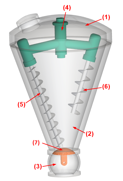
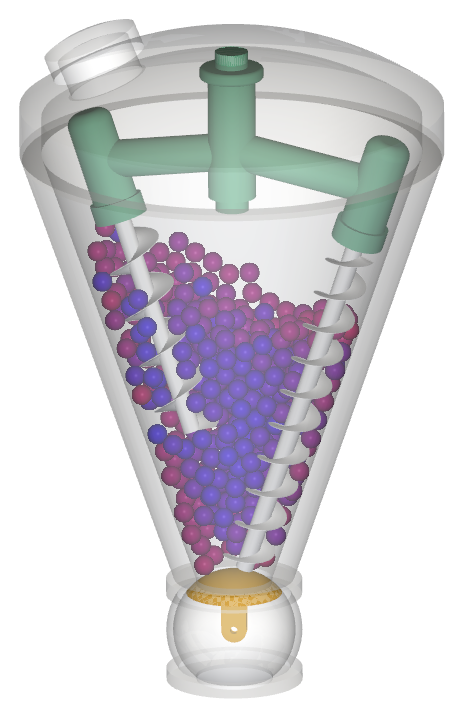
The geometries in this tutorial are composed of:
(1) Lid
(2) Tank
(3) Valve
(4) Central Shaft
(5) Longer Screw
(6) Short Screw
(7) Ball
The .stl files can be found in the tutorial directory.
To get started with this tutorial, do the following:
Download the
dem_tut07_files.zipfile here .Unzip
dem_tut07_files.zipto your working directory.Open Rocky 2025 R2.
Create a new project.
Save the empty project to a location of your choosing.
Use the information in the table that follows to start setting up your Rocky project.
Step Entity Editors Location Parameter or Action Settings A Study 01 Study Study Name Conical Dryer B Physics Physics | Momentum Numerical Softening Factor 0.1 [-] Tip: If you run into settings or procedures in these tables that you are not yet familiar with, please refer to the Rocky User Manual and/or other Tutorials.
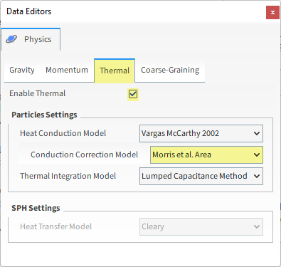
Also for the Physics step, we will be enabling both the Thermal Model and a Conduction Correction Model.
In the previous step, we chose a numerical softening factor lower than 1, which can cause errors within the heat transfer calculations due to the material being modeled softer than it is in reality.
Adding a conduction correction model helps to avoid over-predictions on the contact area in these cases.
Tip: For more information about these models and when to apply them, refer to the Thermal conduction correction models chapter in the DEM Technical Manual.
From the Thermal sub-tab, mark the Enable Thermal checkbox, and then define the Conduction Correction Model (as shown).
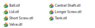
For the Geometries step, we will import the following 7 files in .stl format.
From the Data panel, right-click Geometries and then click Import Wall.
From the Select file to import dialog, navigate to the dem_tut07_files folder that you previously downloaded, find the geometry folder, multi-select all of the 7 files shown above, and then click Open.
From the Import File Info dialog, select "mm" as Import Unit, ensure that the option Convert Y and Z axes is cleared (unchecked), and then click OK.
For the Motion Frames step, we will use nested frames to create a planetary motion, where each screw will rotate around its own axis and the central shaft will rotate the screws around the cone.
In order to create complex motions, Rocky allows new Motion Frames (children) to be linked to previously created Motion Frames (parents).
The children Motion Frames will move together with the parent Motion Frame and will also have their own unique motions.
Note: To enable even more complex nested motions, a child Motion Frame is allowed to have a Local Keep in Place axis while its parent frame is set to Global Keep in Place. However, since we want to have motions with displacement in this simulation (Keep in Place is Disabled). See Tutorial 21 for an exemple of application of this functionality.
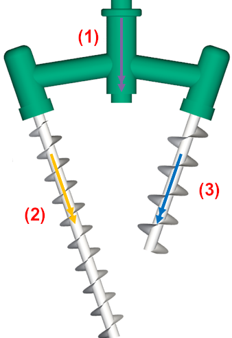
For this case, three separate Rotations will be created:
(1) Central Shaft Motion: This will rotate the whole system (Central Shaft, Longer Screw, and Short Screw) around the dryer's vertical axis.
(2) Longer Screw Motion: This will rotate the longer screw around its own axis.
(3) Short Screw Motion: This will rotate the short screw around its own axis.
Use the information in the table that follows to create the first of these three Motion Frames.
Step Data Entity Editors Location Parameter or Action Settings A Motion Frames Create Motion Frame B Motion Frames ﹂ Frame <01>
Frame Name Central Shaft Motion Add Motion Start Time 1 [s] Type Rotation ▼ Initial Angular Velocity 0, -4, 0 [rev/min] This will be the parent frame upon which the next two frames will depend.
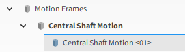
To create a child frame that is dependent upon the parent frame you just created, from the Data panel, right-click Central Shaft Motion, and then select Create Motion Frame.
A new (child) frame called Central Shaft Motion <01> appears nested under the first (parent) frame. Besides the names, the connection between the two frames is also indicated by the name of the parent appearing in bold when the child is selected.
Use the table that follows to define the parameters for this first child Motion Frame.
Step Data Entity Editors Location Parameter or Action Settings A Motion Frames ﹂ Central Shaft Motion <01>
Frame Name Longer Screw Motion Relative Position -0.521, 0, 0 [m] Relative Orientation | Angle -161.045 [dega] Relative Orientation | Vector 0, 0, 1 [-] Add motion Start Time 0.5 [s] Type Rotation ▼ Initial Angular Velocity 0, 57, 0 [rev/min] To create the second dependent (child) frame, use the information in the table that follows.
Step Data Entity Editors Location Parameter or Action Settings A Motion Frames ﹂Central Shaft Motion
Create Motion Frame B Motion Frames ﹂ Central Shaft Motion <01>
Frame Name Short Screw Motion Relative Position 0.463, 0, 0 [m] Relative Orientation | Angle 161.045 [dega] Relative Orientation | Vector 0, 0, 1 [-] Add Motion Start Time 0.5 [s] Type Rotation ▼ Initial Angular Velocity 0, 57, 0 [rev/min]
Once the Motion Frames have been created, each frame must be assigned to a geometry.
Use the information in the table below to complete these assignations.
Step Data Entity Editors Location Parameters or Action Settings A Geometries ﹂ Central Shaft
Wall Motion Frame Central Shaft Motion ▼ B Geometries ﹂ Longer Screw
Wall Motion Frame Longer Screw Motion ▼ C Geometries ﹂ Short Screw
Wall Motion Frame Short Screw Motion ▼ From the Data panel, select Motion Frames.
From the Data Editors panel, click the Preview button.
A new Motion Preview window appears.
For this tutorial, since the geometries have motions with displacement assigned (Keep in Place is Disabled), the movement can be previewed using the Motion Preview window.

Tip: Use the eye icons on the Data panel to hide the Tank and Lid geometries.
The Time toolbar can be used to "play" the preview. The yellow color of the slider indicates that the simulation has not yet been processed.
Note: For this tutorial, no movement will be seen until after 0.5 s.
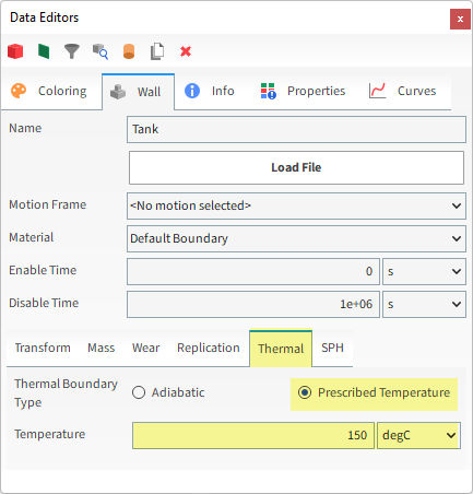
In order to evaluate the heating of the Particles that come into contact with the Tank, Thermal Boundary conditions should be defined for this geometry.
From the Data panel, under Geometries, select Tank.
From the Data Editors panel, select the Wall tab, and then from the Thermal sub-tab, define Thermal Boundary Type and Temperature (and unit).
For the Materials step, two materials will be used: one for all the geometry parts (Default Boundary) and another for the particles (Default Particles).
Use the table below to define the material values for this tutorial.
Step Data Entity Editors Location Parameter or Action Settings A Materials ﹂ Default Boundary
Material Density 7900 [kg/m³] Young's Modulus 2e+11 [N/m²] Thermal Conductivity 400 [W/m.K] Specific Heat 385 [J/kg.K] Poisson's Ratio 0.27 [-] B Materials ﹂ Default Particles
Material Bulk Density 492 [kg/m³] Young's Modulus 2e+08 [N/m²] Thermal Conductivity 311 [W/m.K] Specific Heat 17.56 [J/kg.K] Note: For this tutorial, the Materials Interactions values will be left as default.
For the Particles step, we will create a new spherical particle group.
For the Inlets and Outlets step, we will create a volumetric inlet with thermal properties, which will inject all the particles at once before the simulation starts.
Use the information in the table below to finish setting up your project.
Step Data Entity Editors Location Parameter or Action Settings A Particles Create Particle B Particles ﹂ Particle <01>
Particle | Size (1) Size | Cumulative % 0.08 [m] @ 100 [%] C Inlets and Outlets Create Volumetric Inlet D Inlets and Outlets Inlets and Outlets
﹂ Volumetric Inlet <01>
Volumetric Inlet | Particles Add row (x1) (1) Particle | Mass | Temperature Particle <01> ▼ | 180 [kg] | 25 [degC] Volumetric Inlet | Region Seed Coordinates 0, -0.9, 0 [m] Geometries (All Enabled ("Check All")) Use Geometries to Compute (Enabled) E Solver Solver | Time Simulation Duration 25 [s] Solver | General Simulation Target CPU
In this tutorial, we used Imported Geometries to create the Volumetric Inlet for particles. The Use Geometries to Compute option allows you to easily define a specific region of the simulation within the geometry limits to inject particles. Layers of particles are built around the Seed Point you set, until either the Mass value is reached, or the Region is filled. This allows you to control if you want the interior of an imported geometry to be partially or completelly filled with particles.
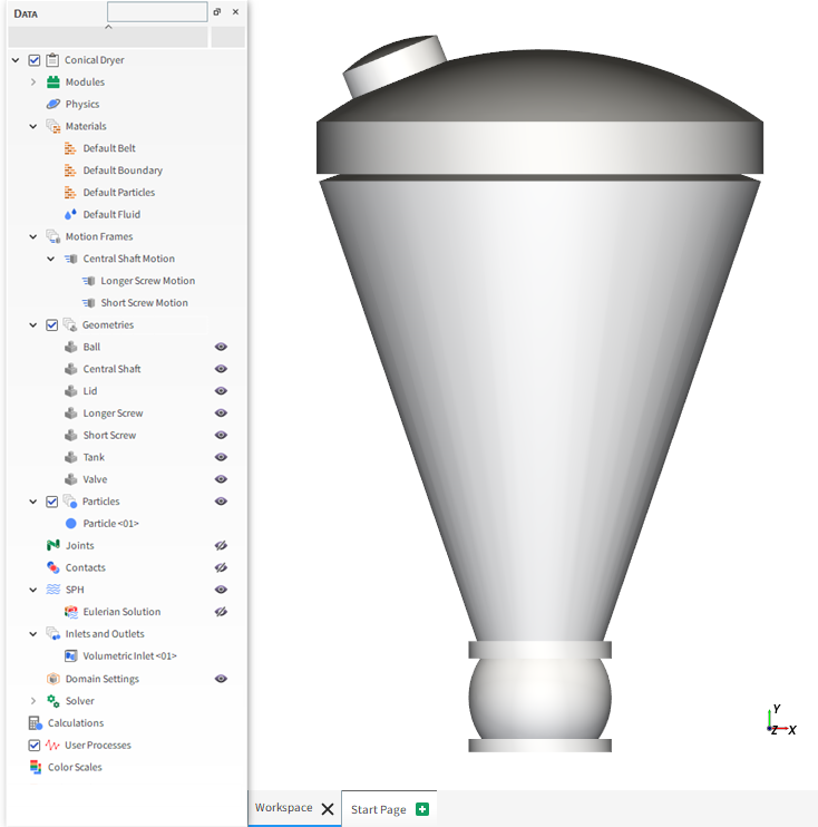
With a 3D View window opened, your Data panel and Workspace should look similar to the below image.
From the Solver entity, click Start.
The Simulation Summary screen appears (as shown), then processing begins.
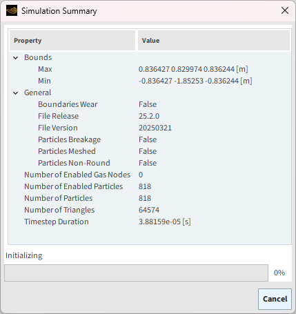
Tip: You can use the Auto Refresh checkbox to view in a 3D View window the results during processing.
This completes Part A of this tutorial, in which Rocky was used to set up and process a thermal simulation of a Conical Double Screw Vacuum Dryer.
During this tutorial, it was possible to:
Use Motion Frames to set up and preview complex, nested motions
Define basic Thermal Modeling parameters for materials and geometries
What's Next?
If you completed this tutorial successfully, you are ready to move on to Part B and post-process this project.
The main purpose of this tutorial is to learn how to analyze conductive heat transfer within the Conical Double Screw Vacuum Dryer simulation we created in Part A.
You will learn how to:
Use Camera Presets to save and apply exact views
Export project post-processing settings
View and plot particle temperature
Track an individual particle
And you will use these features:
Custom Presets toolbar
3D View windows
Export Project Context
Properties
Color Scale
Cell Inspection User Process
Important: This ADVANCED tutorial contains fewer details, screenshots, and procedures than other Rocky tutorials.
An ADVANCED tutorial is designed for users who are more familiar with the Rocky user interface (UI), and already have a good understanding of the common setup and post-processing tasks.
If you do not already have this level of familiarity, it is recommended that you complete at least Tutorials 01- 05 before beginning this one.
If you completed Part A of this tutorial, ensure that Rocky project is open. (Part B will continue from where Part A left off.)
If you did not complete Part A, do all of the following:
Download the
dem_tut07_files.zipfile here .Unzip
dem_tut07_files.zipto your working directory.Open Rocky 2025 R2.
Important: To make use of the Rocky project file provided, you must have Rocky 2025 R2 or later. If you have an earlier version of Rocky, please upgrade Rocky to the latest version, or complete Part A from scratch.
From the Rocky program, click the Open Project button, find the dem_tut07_files folder, then from the tutorial_07_A_pre-processing folder, open the tutorial_07_A_pre-processing.rocky file.
Process the simulation. (From the Data panel, select Solver and then from the Data Editors panel, click the Start button.)
For this tutorial, we will define three specific 3D View Presets of the Dryer geometry: Full View, Shaft View, and Valve View.
A preset enables you to save the exact rotation (tilt), magnification (zoom), and location (pan) settings you have defined in a 3D View.
In this way, you can reuse those exact views for other analyses in the same project.
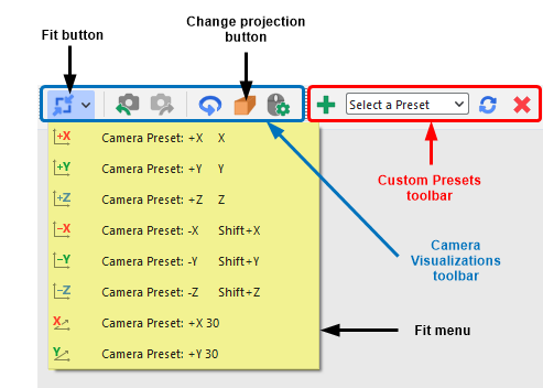
You can define 3D Views using the keyboard, mouse or the Camera Visualization toolbar (shown in blue).
For this tutorial, we will use the Fit menu (shown in yellow) and mouse to change our 3D View, and will then use the Custom Preset toolbar (shown in red) to save our views for reuse later.
Let's start by making the Full View preset.
From the Window menu, click New 3D View.
By default, the view is centered and oriented to the +Z axis. Let's change it as follows:
With the new window selected, ensure the Change projection button is set to Orthogonal (as shown).

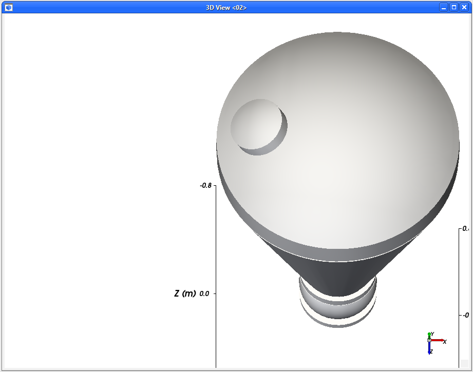
Find the Fit menu, and then select Camera Preset: -Z.
Use your mouse to make the window approximately square.
Select the Fit button (or click R) to reorient the geometry in the center of the window.
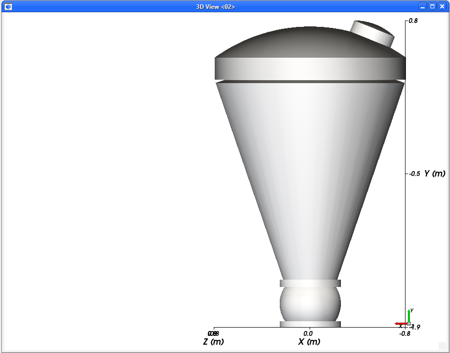
Use your mouse's center wheel to zoom (increase magnification) into the view as much as you can while keeping all the parts in view.
Use your mouse's right button to drag the geometry towards the right side of the window, leaving a empty area on the left.
The results are shown below.
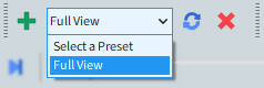
With your new view changed (as shown), from the Custom Presets toolbar, click the Add preset button (green plus) (as shown).

From the Create new preset dialog, enter the name (as shown) and click OK.
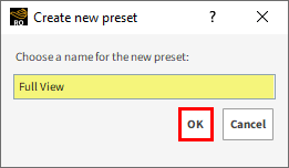
The new Full View preset is listed in the toolbar.
Now, let's create the Shaft View preset:
With the same 3D View window selected, from the Fit menu, select Camera Preset: +Y 30.
Use your mouse's center wheel to zoom (increase magnification) into the view as much as you can while keeping all the parts still within view.
Use your mouse's right button to drag the geometry towards the right side of the window, leaving an empty area on the left (results shown).
From the Custom Presets toolbar, click the Add preset button (green plus).
From the Create new preset dialog, enter the name (as shown) and click OK.

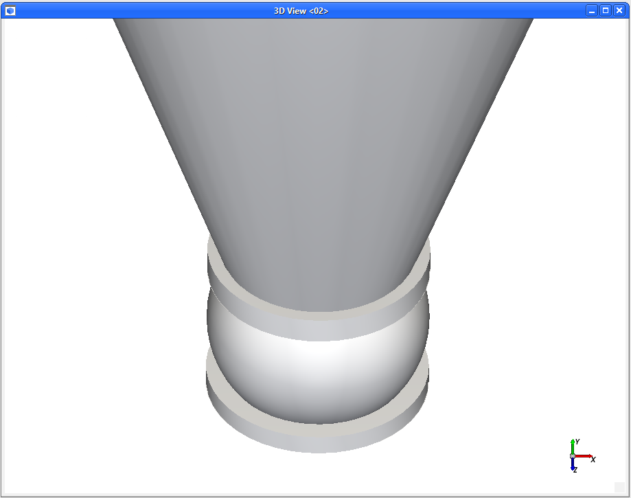
Finally, let's create the Valve view preset:
Within the same 3D View window, use your left mouse button to rotate the view straight up until the Y (green) and Z (blue) axes are both pointing towards you.
Click the Fit button.
Use your mouse's center wheel to zoom into the view until the tank touches both sides of the window.
Use your mouse's right button to drag the geometry up until the valve is fully in view and only the bottom third of the tank is visible. (Results shown.)
From the Custom Presets toolbar, click the Add preset button (green plus).
From the Create new preset dialog, enter the name (as shown) and click OK.
Next, create two more 3D View windows (Ctrl+D) and apply the other two presets to those.
You should now have three separate windows, each with a different preset view (as shown).
Now that these views and windows are set up exactly the way we want, let's export that setup criteria so that we can re-use it in a similar project later.
When you choose to Export project context, Rocky saves in a rocky_template file (or to the clipboard) setup information about all the following items you have defined in your project:
3D View windows
most User Processes
Workspace tabs
Limitations: This method does not currently export setup information for the following:
Windows: Plot, Histogram, Motion Preview, nor Particles Details
User Processes: Cell Inspector, Particle to Contact, nor Contact to Particle
Before we start, let's organize the windows on our Workspace.
From the View menu, ensure Windows is enabled.

From the Windows panel, use the checkboxes to disable all but the 3D View windows (as shown).
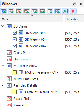
From the Window menu, select Tile 2 Columns (as shown).

Your Workspace should now contain only neatly organized 3D View windows.

From the File menu, point to Export project context, and then click To file.
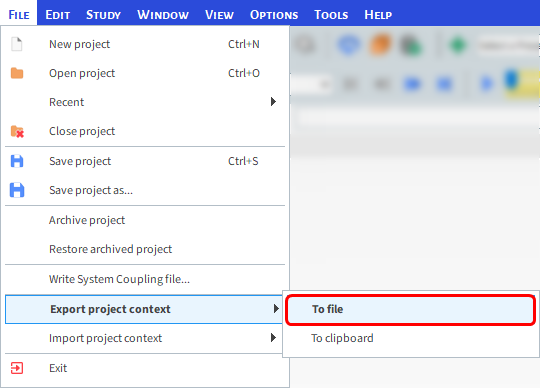
From the Save project context dialog, choose a location and enter a File name for the .rocky_template file, and then click Save.
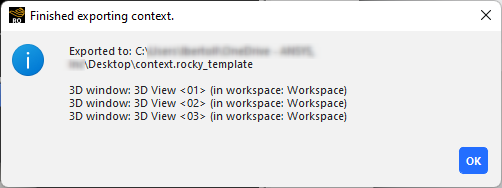
The Finished exporting context window appears, confirming the items exported (as shown).
When you are ready to re-use this setup information, open a similar project, and then from the File menu, point to Import project context, click From file, navigate to and select the .rocky_template file you want, and then click Open.
The setup items you exported will appear in your project.
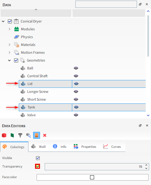
For the next analysis, let's use the Full View preset with transparent geometries.
Select the 3D View window that is showing the Full View preset. (Or, from any other 3D View window, switch to that view by selecting Full View from the Custom Presets toolbar.)
From the Data panel, under Geometries multi-select the Lid and Tank geometry components.
From the Data Editors panel, select the Colorings tab, and then enable the Transparency checkbox (as shown).
We can analyze properties data like temperature by coloring simulation components by property in the 3D View window.
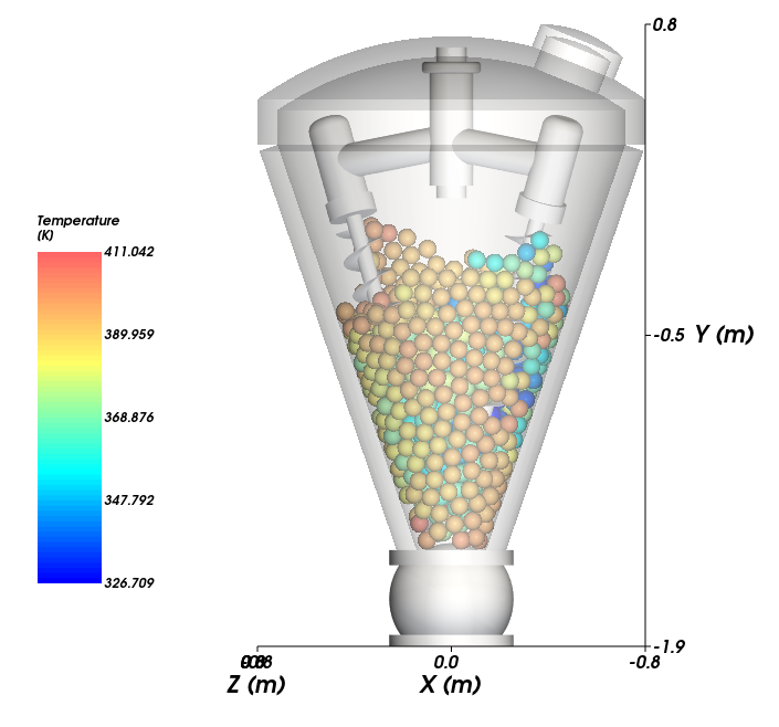
From the Data panel, select Particles and then from the Data Editors panel, select the Properties tab.
Drag and drop the Temperature property (available only when the Thermal Model is enabled) to the 3D View window.
Rocky will create a Color Scale using the default color scheme and limits based upon the minimum and maximum values of the selected Property at the given time.
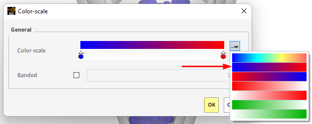
To change the display options, right-click the Color Scale and then select Edit. This shows options from the Coloring tab on the Data Editors panel.
From the Coloring tab, edit the color scheme by clicking on the ... button next to the Color-scale bar.
In the Color-scale dialog that appears, a predefined Color-scale can be selected or a custom one created by moving and/or changing the color of the dots. For this tutorial, click the ... button and select the blue-to-red color scale (as shown), and then click OK.
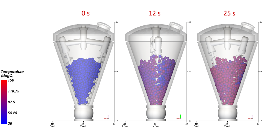
Back on the Coloring tab, the Limits options can be set manually by selecting User Defined from the drop down list. For this tutorial, define the Limits values and the Color-scale unit (as shown).

Use the Time toolbar to display the Temperature at different Output times.
The Temperature property can also be used in plot to analyze the uniformity of the Particles being heated.
From the Window menu, click New Time Plot (or press Ctrl+T).
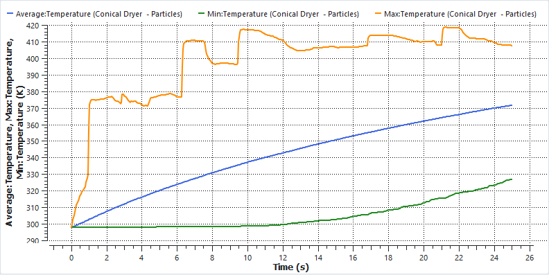
Use the information in the table below to define the Time Plot.
Step Item Location Parameter or Action Settings A Particles Properties | Temperature Drag and drop onto the Time Plot window B Select the Statistics to Plot (dialog box) Min (Enabled) Max (Enabled) Average (Enabled) Right-click the Plot grid, point to Axes Layout, and then select By Quantity.
Tip: From the Select The Statistics to Plot dialog box, clear any other checkbox that is possible enabled.
The results are shown below.
It may be useful to correlate simulation results with instrumentation data, such as a probe on the geometry or a particle tracer.
The Cell Inspector User Process allows you to evaluate results on a single selected Triangle (Geometries), Particle, or Eulerian Bin.
For this tutorial, two Particles will be located when motion starts and then their Temperatures tracked over time: One at the top-center of the Cone and the other at the bottom. (Note that the actual ID of your particles might differ slightly.)

To find the two particles you will use:
Find (or create from new) the 3D View window you created earlier that uses the Shaft view Preset, and the other that uses the Valve view Preset.
For both windows, turn the Particles color to gray, and then make the Lid and Tank Geometries transparent.
From the Time toolbar, set the output time to 0 s.
With the Shaft view window selected, from the Data panel right-click Particles, point to Processes, and then click Cell Inspector.
From the Data Editors panel, on the Coloring tab (for the Inspector <01> entity), change the Node color to red.
From the Inspector tab, change the Name (as shown) and then use the arrows (or type numbers) on the Particle ID list box to show on the 3D View the location of individual particles until you find one at the top of the Cone (in this tutorial, ID 802).


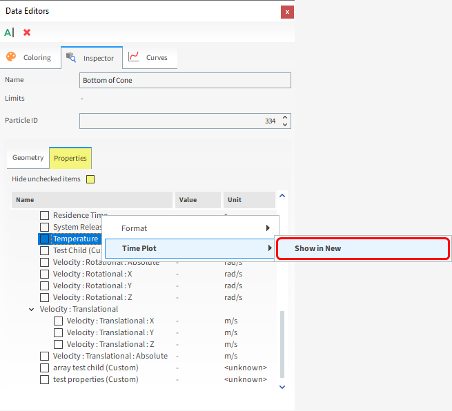
With the Valve view window selected, repeat this process to create another Cell Inspector User Process identifying a particle at the bottom of the Cone (in this tutorial, ID 334). Change the Name of this process to Bottom of Cone.

From the Properties sub-tab, clear the Hide unchecked items checkbox (as shown).
From the Properties sub-tab, right-click Temperature, point to Time Plot, and then click Show in New.
From the Data panel, under User Processes, select the Top-center of Cone inspector.
From the Properties sub-tab, ensure the Hide unchecked items checkbox is still cleared.
From the Properties sub-tab, right-click Temperature, point to Time Plot, and then click Show in Current.
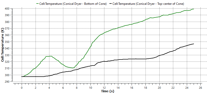
The exact behavior of your two particles will likely be different than the ones shown here. But for example, here's what we can observe from this particular plot:
Up until 4 seconds, the particle at the bottom of the cone experienced heating due to wall contact. After this, it experiences some heat loss due to conduction with cooler neighboring particles, until it starts to heat up again around 7 seconds.
The particle at the top-center of the cone remained more in the middle of the equipment and increased its temperature more steadily.
By the end of the simulation, both particles have the temperature increased.
This completes Part B of this tutorial, in which Rocky was used to post-process a thermal simulation of a Conical Double Screw Vacuum Dryer.
During this tutorial, it was possible to:
Use Camera Presets to save and apply exact views
Save those views for use in similar projects by Exporting project context
Use Properties to evaluate particle temperature and uniformity parameters
Create tracers using the Cell Inspector User Processes to evaluate individual particle behavior
What's Next?
If you completed this tutorial successfully, then you are ready to move on to next tutorial.