


(Part A) Set up and process a Drop Weight Test (DWT) using free body translations and the Ab-T10 breakage model.
(Part B) Learn how to evaluate the PSD and total amount of broken fragments.
The purpose of this tutorial is to set up and process a Drop Weight Test (DWT) and learn how to change Ab-T10 breakage parameters in order to adjust the particle breakage properties for future Rocky simulations.
Important: Even though this tutorial involves running only one drop-weight test, the random nature of the expected results dictates that the average of many multiple tests should be used as the basis for any real-life calibrations.
Note: We will post-process this simulation in Part B.
You will learn how to:
Create a circular surface
Define a free body translation motion
Enable the Ab-T10 breakage model
And you will use these features:
Motion Frames
Particle Breakage
This tutorial assumes that you are already familiar with the Rocky user interface (UI) and with the project workflow.
If this is not the case, please refer to Tutorial 01 – Transfer Chute for a basic introduction about Rocky usage before beginning this tutorial.
Tip: If you are unsure which version of Rocky you have, ask your IT department, or contact Rocky Support for assistance.
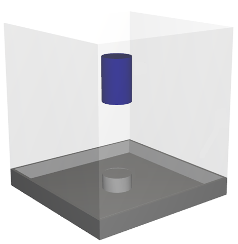
The geometries in this tutorial are composed of:
(1) Drop Weight
(2) Anvil
(3) Walls
In the tutorial directory, the .stl files can be found.
To help you determine the breakage parameters to use for your simulated material, there are experimental tests that can be done, such as the JK Drop Weight Test (DWT).
The DWT involves releasing a drop weight over a rock sample from a specific height and then observing the resulting behavior.
By using this method on your real-world material, you can:
Calculate the mass of fragments that have sizes less than 1/10th of the original size.
Calculate the impact specific energy.
The results can then be used to calibrate particle parameters in Rocky to achieve similar breakage results in your simulations.
Important: Unlike the single run demonstrated in this Tutorial, an average of many multiple Rocky tests should be used as the basis for any real-life breakage calibrations.
To start the tutorial, let's create a new project:
Download the
dem_tut05_files.zipfile here .Unzip
dem_tut05_files.zipto your working directory.Open Rocky 2025 R2. (Look for Rocky 2025 R2 in the Program Menu or use the desktop shortcut.)
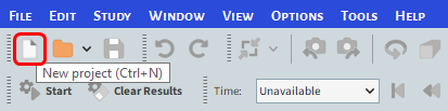
From the Rocky program, click the New Project button, or from the File menu, click New Project (Ctrl+N).
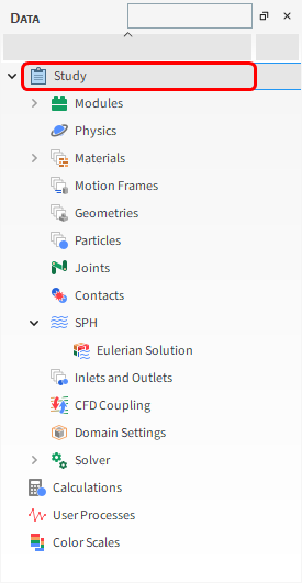
The Study entity covers the first step of the simulation setup. The purpose is to define any useful information for the project.
From the Data panel, click Study.
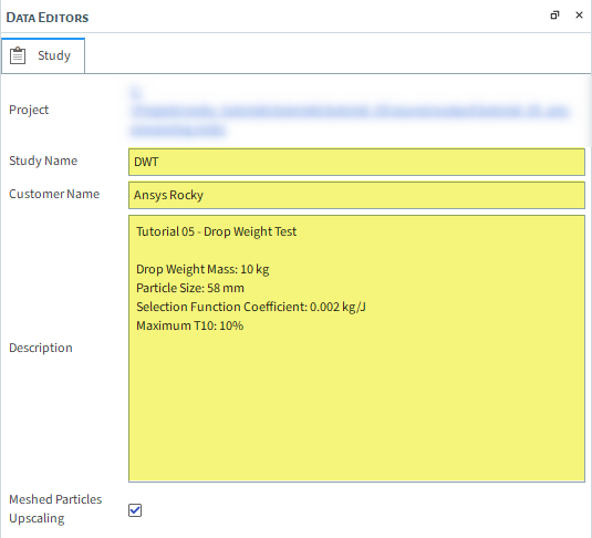
From the Data Editors panel, enter the Study Name and other project details (as shown).
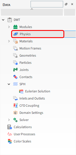
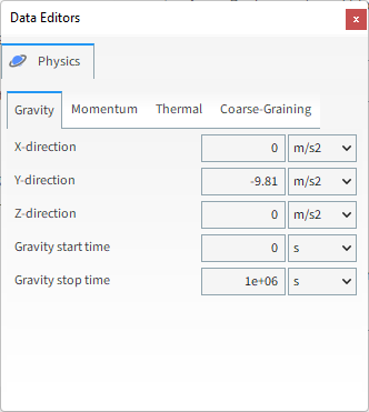
For the Physics step, from the Gravity tab, you are able to define the gravity components and the time during which gravity is applied during the simulation.
For this tutorial, we will use the default values (no changes).
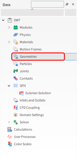
For the Geometries step, we will import wall geometry files in .stl format.
From the Data panel, right-click Geometries and then select Import Wall.
From the Select file to import dialog, navigate to the dem_tut05_files folder that you previously downloaded, find the geometry folder, and then while pressing either the Ctrl or Shift key, multi-select all of the following files, and then click Open:
anvil.stl
dropweight.stl
wall.stl
Save your project now if you have not already done so.
From the Import File Info dialog, select "mm" as Import Unit, ensure that the option Convert Y and Z axes is cleared (unchecked), and then click OK.
The next step is to define a geometry Surface from which to release particles into the domain.
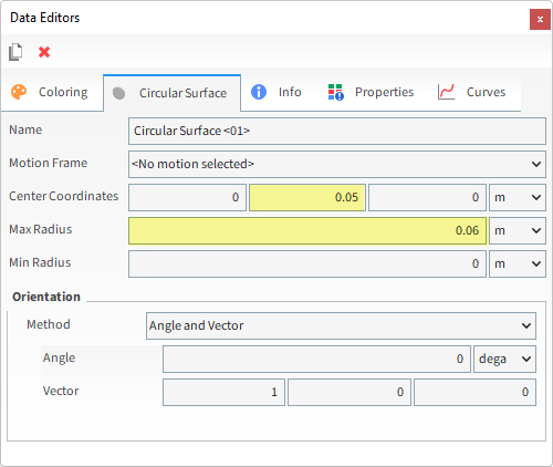
From the Data panel, right-click Geometries and then click Create Circular Surface.
Under Geometries, select the newly created Circular Surface <01>.
From the Data Editors panel, on the Circular Surface sub-tab, define the Center Coordinates and Max Radius.
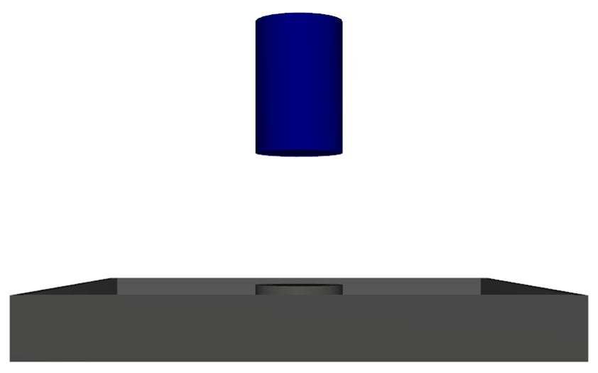
For this test, the drop weight is raised to a prescribed height and then dropped.
The mass will have a free vertical body motion, since the only force will be the weight force (due to gravity).
When the motion Type of Free Body Translation or Free Body Rotation is selected, the following options are available:
Free Motion Direction: Specifies in which directions the geometry can move due to particle forces, which is given in the local coordinates of the frame related to the initial frame orientation.
Free Body Linear Limits and Free Body Angular Limits: Specifies how much the geometry can move in each direction.
Each Motion Frame has its own orientation reference (coordinate system) upon which its movements are based.
The current (i.e., instantaneous) orientation is represented in the Motion Preview window by the axes for the Frame (as shown).
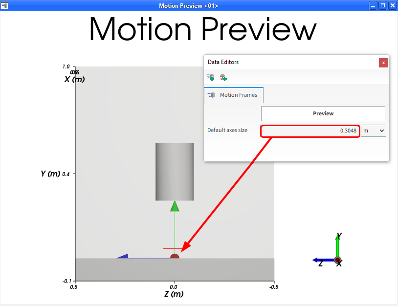
In this version of Rocky, all Frames use only an implicit local reference, which uses the current orientation of the selected Frame to define the next movement.
In this way, the reference is always moving along with the Frame.
Let's look at an example.
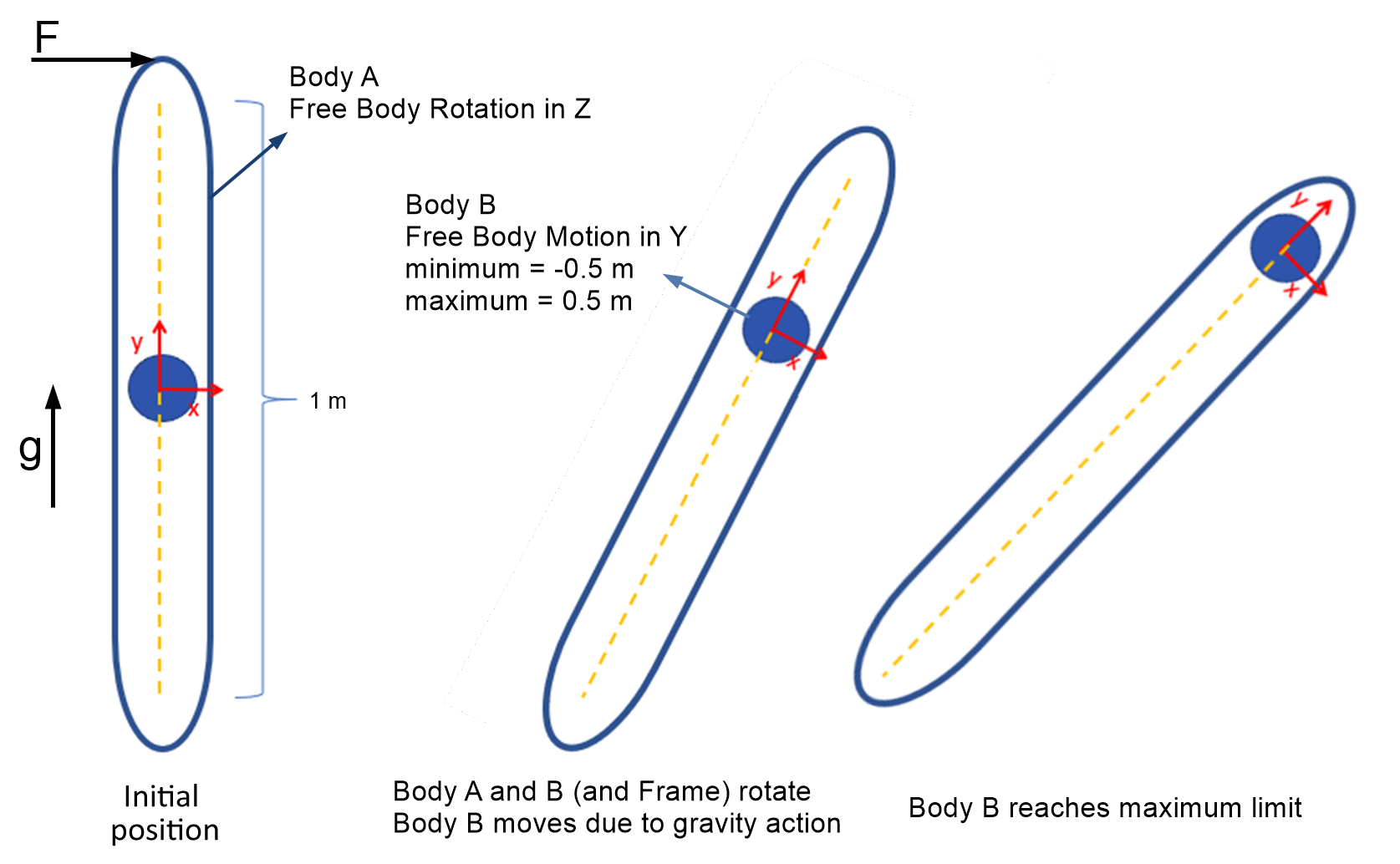
In this example, the rail (yellow dotted line) rotates as the Body A rotates (left image).
The frame's orientation rotates together with Body A.
The gravity is set to the +y direction and a force F is applied on the top of Body A.
As the Free Body Rotation is set to the z direction for Body A, it will be allowed to rotate around its center on the xy plane.
As the Free Body Motion for Body B is set to the y direction, it will be allowed to move along the rail direction (center image).
The maximum free body limit restricts the displacement of the Body B in the local y direction, keeping it inside the rail (right image).
Besides the Frame reference, the orientation of the Frame helps define how the body will behave when it is in motion.
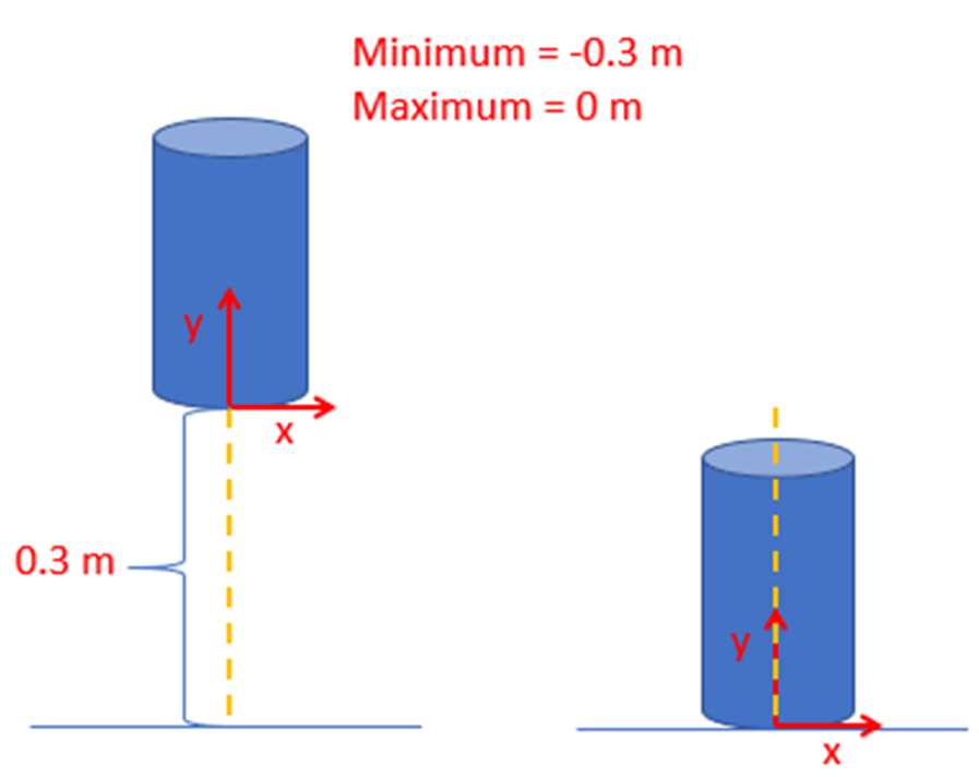
In this next example, the Motion Frame is oriented so that the y axis points upwards.
With the Free Body Motion set to the y direction and the minimum limit in the y set to -0.3 m, the geometry will be able to move freely as much as 0.3 m downwards, stopping when it reaches the bottom.
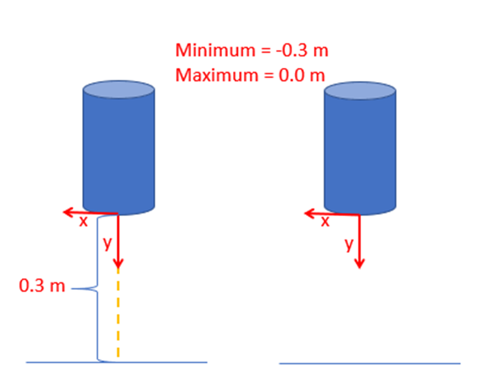
In this next example, the Motion Frame is oriented in the opposite way (the y axis now points downwards).
If the minimum y limit is still set to -0.3 m and the maximum y limit is set to 0 m, the geometry will not move, as it can only move 0 m in the positive y direction.
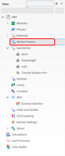
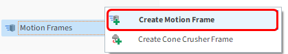
To define a Motion Frame, do the following:
From the Data panel, right-click Motion Frames and then select Create Motion Frame.
From the Data panel, select the newly added Frame <01> entry.
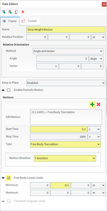
Now we'll define the motion for this frame:
From the Data Editors panel, define the Name: Drop Weight Motion.
Click the green plus button (Add Motion) to create a motion using this frame.
Define Start Time, Type and Motion Direction.
Enable the Free Body Linear Limits checkbox.
Set the Minimum Y limit to ensure that the dropweight stops at the anvil.
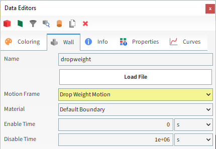
Once the Motion Frame has been created, it must be assigned to the geometry.
From the Data panel under Geometries, select dropweight.
From the Data Editors panel, on the Wall tab, and then select Drop Weight Motion from the Motion Frame drop-down list.
Note: Only effects from gravity forces and not effects from particles, which have yet to be calculated will be displayed for the Free Body Motion in the Motion Preview window.
Once the Free Body Motion is enabled, the mass properties of the moving boundary should be defined.
From the Wall tab, select the Mass sub-tab, and then define the Boundary Mass.
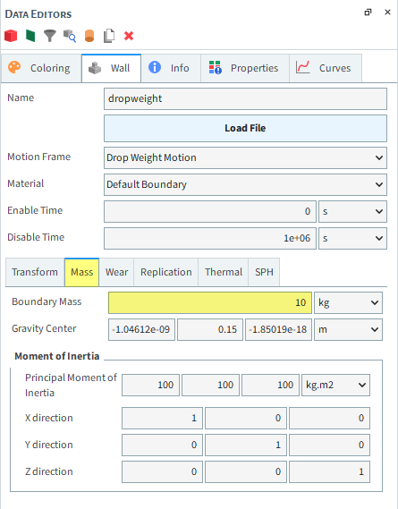
Tip: If Free Body Rotation was used, it would be needed to specify the moment of inertia to correctly account for the angular acceleration and velocity.
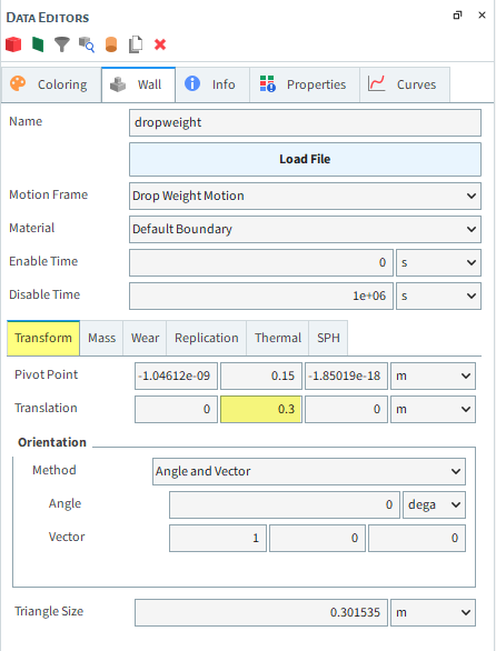
The drop weight will be raised to a prescribed height, according to the experiment to be reproduced.
From the Wall tab, select the Transform sub-tab, and then define Translation.
To visualize the newly created Frame, from the Data panel click Motion Frames and then on the Data Editors click Preview. A new window will appear showing the geometry and the created Frame.
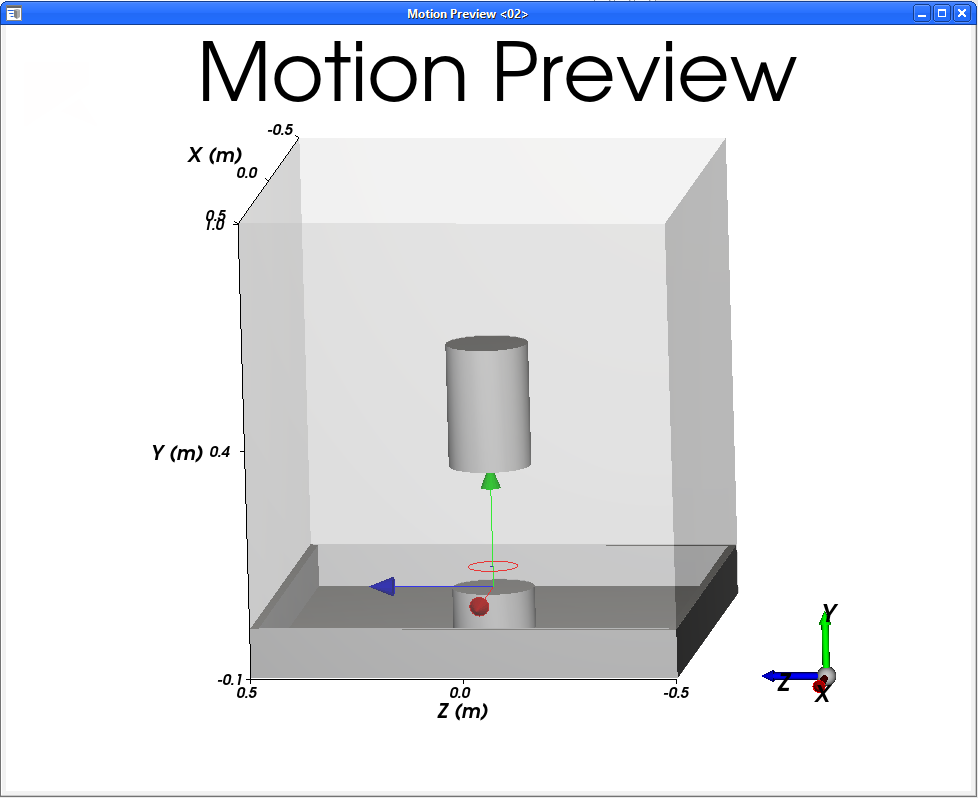
Tip:
To better see all the geometries, enable their Transparency settings from the Geometries Coloring tab.
To better see the Frame's axes, increase the Default axes size parameter from the Motion Frames Data entity.
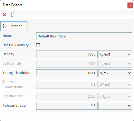
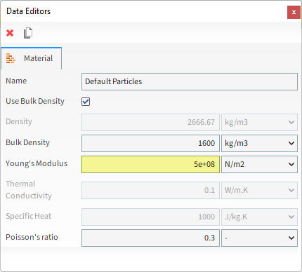
For the Materials step, only two materials will be used: one for all geometry parts (Default Boundary) and another for the particles (Default Particle).
For Default Boundary, keep all the values as default.
For Default Particles, change only the Young's Modulus.
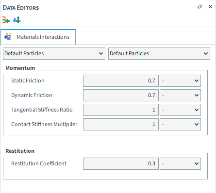
Now let's check the interaction properties for the materials:
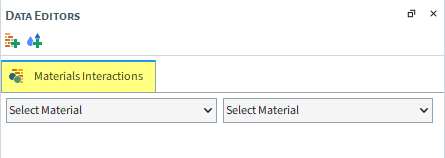
From the Data panel, select Materials. From the Data Editors panel, select Materials Interactions main tab.
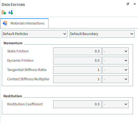
From the left drop-down list, select Default Particles, and from the right drop-down list, select one of its pairs: Default Particles or Default Boundary.
Check the values. We will use the default ones for this tutorial.
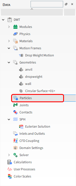
For the Particles step, we will create a new (rock-like) polyhedron-shaped particle group and will define the Ab-T10 breakage parameters for it.
From the Data panel, right-click Particles and then click Create Particle.
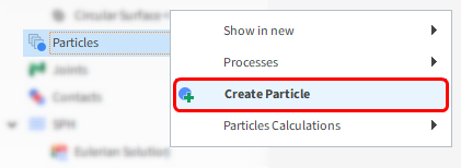
A new particle group is created under Particles.
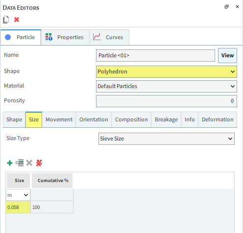
Select the newly created Particle <01> entry.
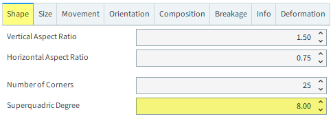
From the Data Editors panel, on the main Particle tab, define the Shape parameter.
From the Size sub-tab, define Size.
From the Shape sub-tab, define the Superquadric Degree.
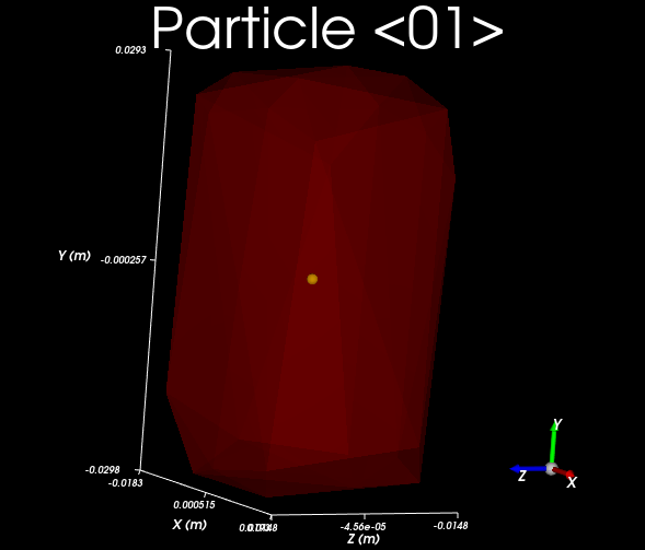
To visualize the newly created particle, click View, next to the particle name.
In this simulation, the Ab-T10 Breakage model (Instant Fragmentation) will be enabled.
This model works with any shaped (non-spherical) Solid particle shape that comes with Rocky (Polyhedron, Briquette, and Faceted Cylinder).
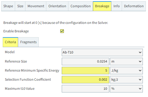
When this model is enabled, the following settings are available on the Breakage | Criteria sub-tab:
Reference Size: The reference size used for measuring the other breakage parameters (experimentally derived).
Reference Minimum Specific Energy: The minimum energy that can lead to the breakage of a reference-sized particle.
Selection Function Coefficient: A measure of the material hardness (known as S in the breakage expression discussed below).
Maximum t10 Value: The maximum mass percentage of particles that can be broken into fragments below 1/10th of the original particle size (known as M in breakage expression discussed below).
In the mining industry, the two values Maximum t10 Value (M) and Selection Function Coefficient (S) are normally not used.
Rather, their product M·S (or more commonly seen as A·b) is used. This is because having a separate breakage probability and product fineness are not as important for understanding the breakage process in most cases only the combined value.
To calculate A·b [ton/kWh], use the following units and expression:
 | (5–1) |
Where
[S] = kg/J
[M] = %
This relation will be valid for Reference Size equal to 1
Shi, F. N.; Kojovic, T. "Validation of a model for impact breakage incorporating particle size effect", International Journal of Mineral Processing, 82-3, p. 156-163. 2007.
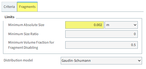
In addition, the following settings are available on the Breakage | Fragments sub-tab:
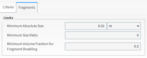
Limits:
Minimum Absolute Size: Smallest size the particle fragments can be at each breakage incident.
Minimum Size Ratio: Smallest size the particle fragments can be at each breakage incident, relative to the parent particle (either a whole particle or a fragment).
Minimum Volume Fraction for Fragment Disabling: Defines the minimum volume fraction that a broken particle (fragment) can have before being considered too small to be included in calculations. Note: In these cases, the too-small fragments will be removed from the system.
Distribution model: The type of fragment size distribution used in the model.
To define the breakage model for the Particle <01> group, do the following:
From the Particle tab, on the Breakage sub-tab, check the Enable Breakage checkbox.
From the Criteria sub-sub-tab, define Reference Minimum Specific Energy and Selection Function Coefficient.
From the Fragments sub-sub-tab, define the Minimum Absolute Size.
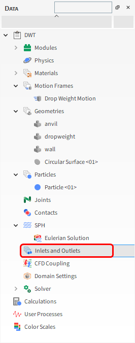
For the Inlets and Outlets step, we will create a Particle Inlet and then set our inlet as the location from which we want particles to enter the simulation.
From the Data panel, right-click Inlets and Outlets and then select Create Particle Inlet.
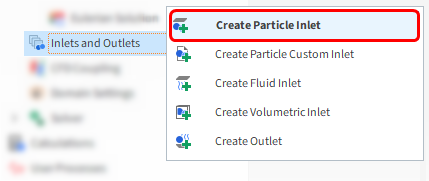
A new entry is created under Inlets and Outlets.
Select the newly created Particle Inlet <01> entry and then from the Data Editors panel, modify the parameters as specified below.
From the Entry Point drop-down list, select Circular Surface <01>.
From the Particles sub-tab, click the Add (green plus) button to add a new mass flow rate row.
From the Particle column, select Particle <01> from the drop-down list and then define the Mass Flow Rate in t/h.
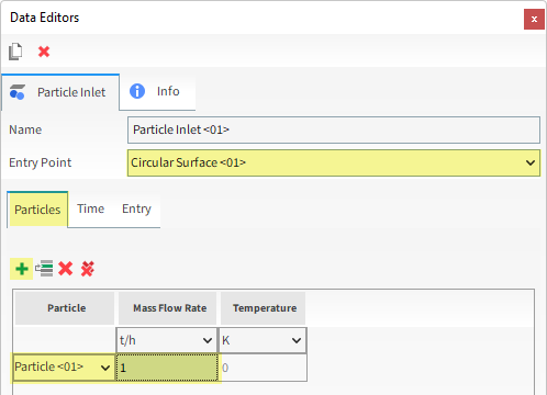
Note: For this simulation, the small Mass Flow Rate combined with the small injection time limits the inlet to a single particle only, which is the minimum amount that Rocky can release.
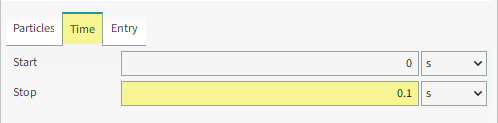
From the Time sub-tab, enter the Stop time.
Now let's set up the solver:
From the Data panel, click Solver and then from the Data Editors panel, select the Solver tab.
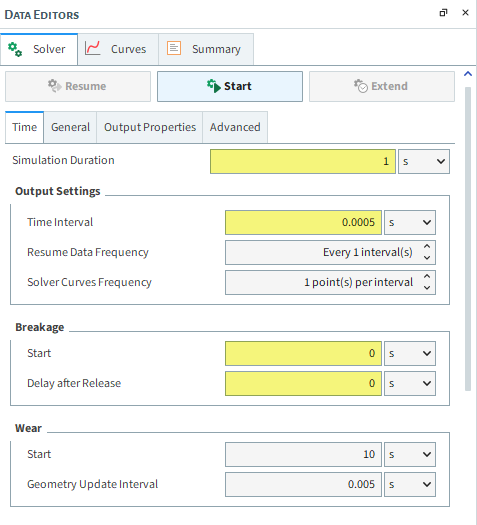
From the Time sub-tab, define the: Simulation Duration, and Output Frequencies: Simulation.
Note: The smaller Output Frequency will help us to better visualize the particle breaking.
Under Breakage, define also the Start and Delay after Release values (as shown).
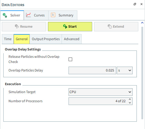
From the General sub-tab, under Execution, select CPU (or GPU/Multi GPU) as Simulation Target, and then set the Number of Processors (or Target GPU(s)).
Click Start.
Once you click Start, the Simulation Summary window will be displayed.
Once initialization is complete, this screen will close automatically and Rocky will process your simulation.
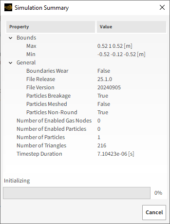
Tip: You can also review this information from the Solver | Summary tab.
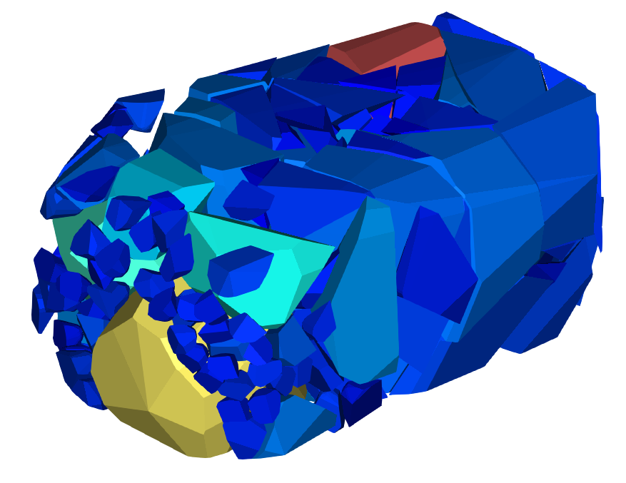
To visualize the simulation as it's processing:
From the Window menu, click New 3D View.
Tip: Hide or make Transparent the wall geometry to better visualize the particle.
Click the Refresh button (or use the Auto Refresh checkbox) to see the results during processing.
The speed of the simulation depends on various factors such as:
Number of mesh elements used to define the geometry
Number of contacts in the simulation domain at any time
Smallest particle size and material stiffness
The particle shape and the number of vertices used to define the shape
Frequency of file output
This completes Part A of this tutorial.
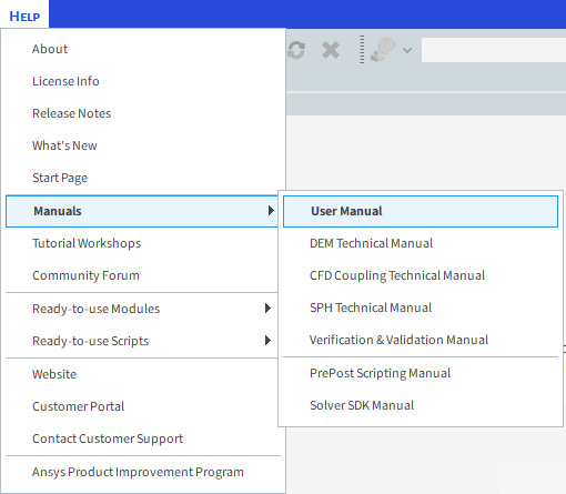
For further information on any topic presented, we suggest searching the User Manual, which provides in-depth descriptions of the tools and parameters.
To access this manual, from the main Toolbar click Help, point to Manuals, and then click User Manual.
Rocky was used to simulate a single-particle Drop Weight Test (DWT) breakage experiment.
Note: The average of many multiple tests should be used as the basis for any real-life calibrations.
During this tutorial, it was possible to:
Create a circular Inlet.
Use Motion Frames to set up a freely translating motion.
Define basic Ab-T10 Breakage Model parameters for a Polyhedron-shaped particle.
What's Next?
Now that you have set up and processed this simulation, you are ready to move on to Part B and post-process this project.
The purpose of this tutorial is to learn how to post-process the Drop Weight Test (DWT) Ab-T10 breakage simulation we set up and ran in Part A.
Note: Even though Part A of this tutorial involved running only one drop-weight test, the random nature of the results expected dictates that the average of many multiple tests should be used as the basis for any real-life calibrations.
You will learn how to:
Evaluate the Particle Size Distribution (PSD) and total amount of the broken fragments
Evaluate the free body motion and displacement of the drop weight
And you will use these features:
Histograms
Time Plots
Multi Time Plots
This tutorial assumes that you are already familiar with the Rocky user interface (UI) and with the project workflow.
If this is not the case, please refer to Tutorial 01 – Transfer Chute for a basic introduction about Rocky usage before beginning this tutorial.
Tip: If you are unsure which version of Rocky you have, ask your IT department, or contact Rocky Support for assistance.
If you completed Part A of this tutorial, ensure that Rocky project is open. (Part B will continue from where Part A left off.)
If you did not complete Part A, do all of the following:
Download the
dem_tut05_files.zipfile here .Unzip
dem_tut05_files.zipto your working directory.Open Rocky 2025 R2. (Look for Rocky 2025 R2 in the Program Menu or use the desktop shortcut.)
From the Rocky program, click the Open Project button, find the dem_tut05_files folder, then from the tutorial_05_A_pre-processing folder, open the tutorial_05_A_pre-processing.rocky file.
Process the simulation. (From the Data panel, select Solver and then from the Data Editors panel, click the Start button.)
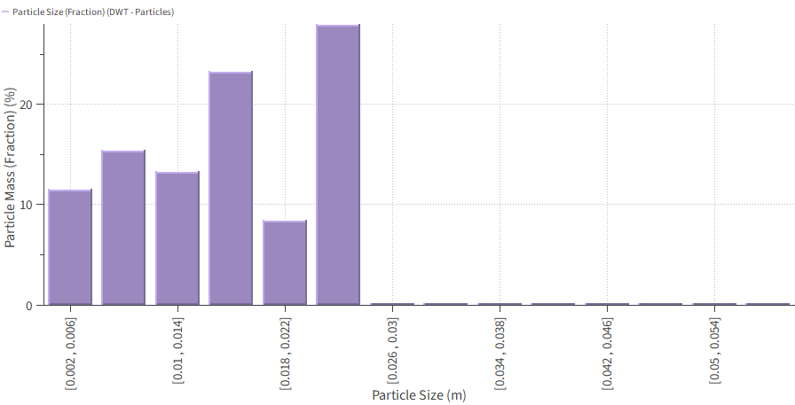
To evaluate the fragments' Particle Size Distribution (PSD), a Histogram will be used.
From the Window menu, click New Histogram, or use the shortcut Ctrl+H.
From the Data panel, select Particles and then from the Data Editors panel, from the Properties tab drag and drop Particle Size within the Histogram window.
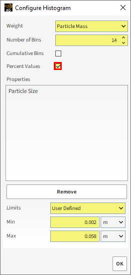
To improve the resulting plot, from the top left of the Histogram window, click the Configure histogram icon.
From the Configure Histogram dialog, change the parameters and then click OK.
The resulting histogram is displayed below.
Note: These values correspond to the last output time (1 s).
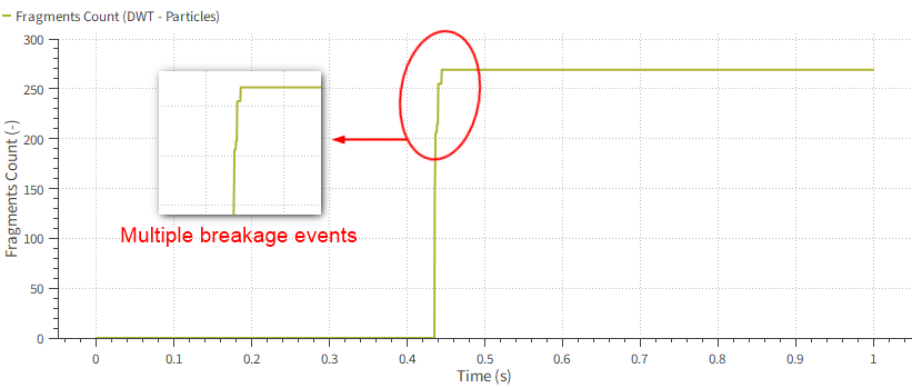
The number of resulting fragments can be evaluated using a Time Plot and creating a curve of the Fragments Count.
From the Window menu, click New Time Plot (Ctrl+T).
From the Data panel, select Particles and then from the Data Editors panel, from the Curves tab drag and drop Fragments Count within the plot. Results are shown.
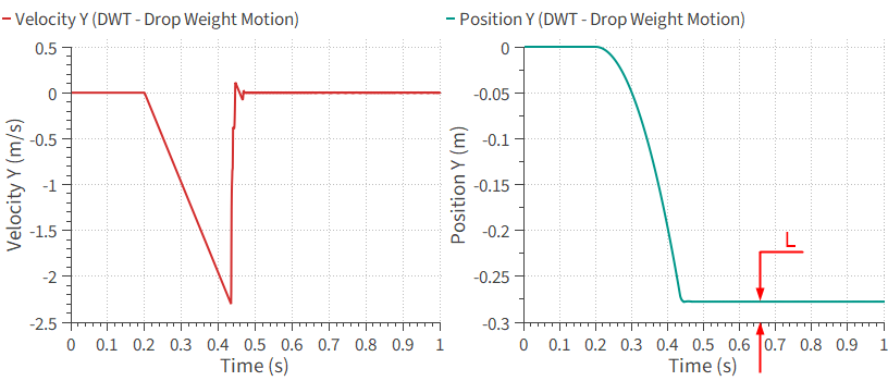
Lastly, we will use a Multi Time Plot to evaluate both the velocity and the displacement of the drop weight.
From the Window menu, select New Multi Time Plot, or use the shortcut Ctrl+M.
From the Data panel, under Motion Frames, select Drop Weight Motion.
From the Data Editors panel, select the Curves tab and then drag and drop Velocity Y within the Multi Time Plot window.
Select Position Y, drag it to the plot area, press and hold the Ctrl key, and then drop it within the same Multi Time Plot window.
The resulting plots are shown below.
You can open a 3D View to better understand the resulting Multi Time Plot.
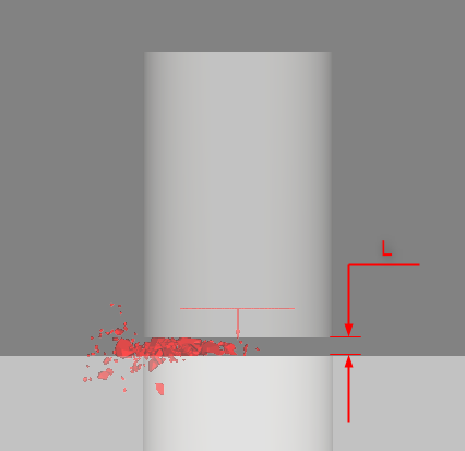
Note how the distance L corresponds to the difference between the Free Body Motion Limits and the final dropweight position.
Also note that it happens because the dropweight stands on a fragment of the particle in the final output times. Otherwise, the dropweight would fall for 0.3 m (corresponding to the Frame Limits).
This completes Part B of this tutorial.
For further information on any topic presented, we suggest searching the User Manual, which provides in-depth descriptions of the tools and parameters.
To access this manual, from the main Toolbar click Help, point to Manuals, and then click User Manual.
Rocky was used to post-process the single-particle Drop Weight Test (DWT) breakage experiment we ran in Part A.
Note: The average of many multiple tests should be used as the basis for any real-life calibrations.
During this tutorial, it was possible to:
Use Time Plots and Histograms to evaluate the resulting Particle Size Distribution (PSD) and fragment amount generated after breakage.
Set up a Multi Time Plot to evaluate the free body motion of the drop weight.
What's Next?
If you completed this tutorial successfully, then you are ready to move on to next tutorial.