


(Part A) Learn how to define vibration motions for a vibrating screen.
(Part B) Analyze the screening efficiency of a vibrating screen using User Processes, custom Curves, and Time Plot functions.
(Part C) Learn how to make optimization analysis via optiSLang for the screening efficiency of a vibrating screen.
The main purpose of this tutorial is to learn how to define vibration motions for a vibrating screen.
You will learn how to:
Define a vibration motion
Define a particle size distribution (PSD)
Set custom domain limits
Extend the simulation duration
And you will use these features:
Motion Frames
This tutorial assumes that you are already familiar with the Rocky user interface (UI) and with the project workflow.
If this is not the case, please refer to Tutorial 01 – Transfer Chute for a basic introduction about Rocky usage before beginning this tutorial.
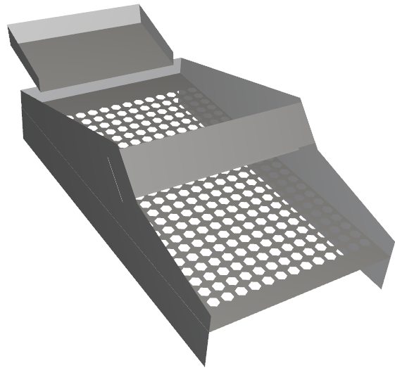
The geometry in this tutorial is composed of:
Vibrating Screen
In the tutorial directory, the .stl file can be found.
To begin the steps for this tutorial, do the following:
Download the
dem_tut03_files.zipfile here .Unzip
dem_tut03_files.zipto your working directory.Open Rocky 2025 R2. (Look for Rocky 2025 R2 in your Program Menu or use the desktop shortcut.)
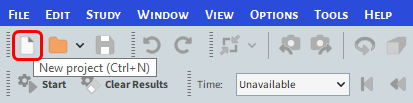
From the Rocky program, click the New Project button, or from the File menu, click New Project (Ctrl+N).
The Study entity covers the first step of the simulation setup. The purpose is to define any useful information for the project.
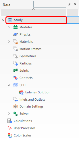
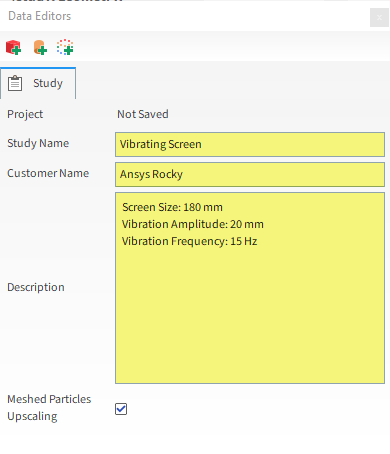
From the Data panel, click Study.
From the Data Editors panel, edit the parameters (as shown).
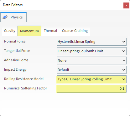
For the Physics step, we will set the model for rolling resistance and then lower the numerical softening factor to reduce the simulation time.
Important: Lowering the numerical softening factor may cause excessive overlaps between particles and between particles and boundaries.
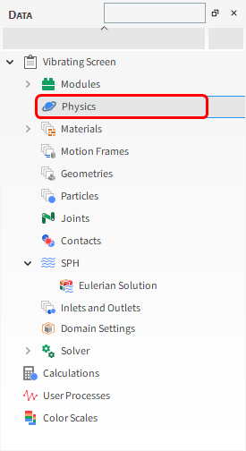
From the Data panel, select Physics.
From the Data Editors panel, select the Momentum sub-tab, and then set the Rolling Resistance Model and the Numerical Softening Factor.
For the Geometries step, we will import a Wall geometry file in .stl format, and then add a Surface to associate later with an Inlet and release particles into the domain.
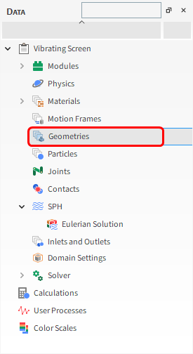
From the Data panel, right-click Geometries and then click Import Wall.
From the Select file to import dialog, navigate to the dem_tut03_files folder that you previously downloaded, find the geometry folder, select the following file, and then click Open:
screen.stl
(Save your project now if you have not already done so).
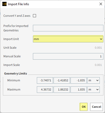
From the Import File Info dialog, select "mm" as Import Unit, ensure that the option Convert Y and Z axes is cleared, and then click OK.
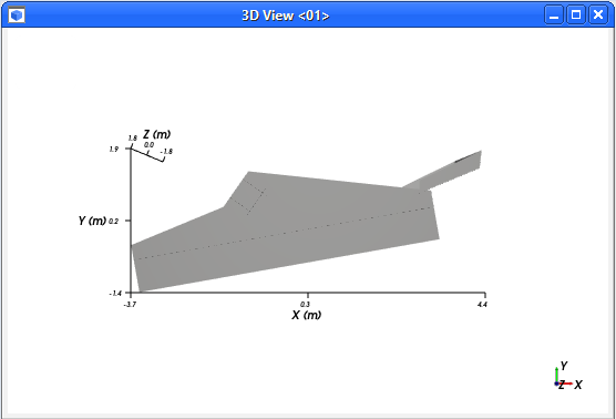
After importing the geometry, you can visualize it in a new 3D View window. To do this:
Drag and drop the Geometries entity from the Data panel onto the Workspace. A new 3D View window appears showing the geometries that you imported (as shown).
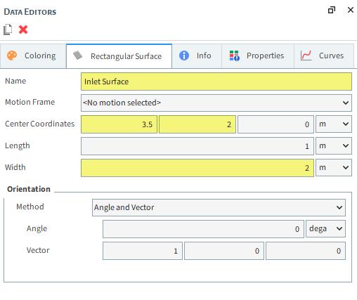
Now let's define the inlet Surface:
From the Data panel, right-click Geometries and then click Create Rectangular Surface.
Under Geometries, select the newly created Rectangular Surface <01> entry.
From the Data Editors panel, on the Rectangular Surface sub-tab, define: Name, Center Coordinates and Width (as shown).
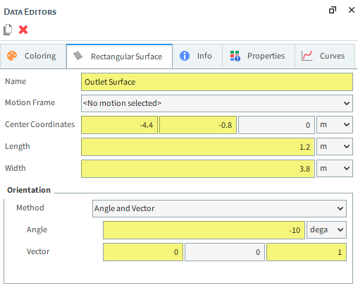
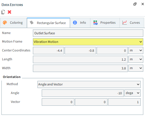
Let's define the outlet Surface:
From the Data panel, right-click Geometries and then click Create Rectangular Surface.
Under Geometries, select the newly created Rectangular Surface <02> entry.
From the Data Editors panel, on the Rectangular Surface sub-tab, define: Name, Center Coordinates, Length, Width and Orientation (as shown).
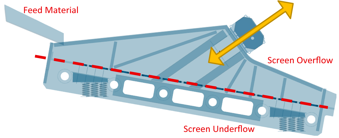
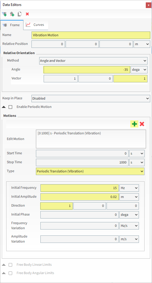
For the Motion Frames step, a single-axis Periodic Translation (Vibration) movement (shown in yellow) will be defined within a Motion Frame and then applied to the screen geometry.
In order to evaluate the separation efficiency of the screen, the following items will be compared:
Feed Material: Particle mass that was originally injected.
Screen Overflow: Particle mass that doesn't make it through the vibrating screen.
Screen Underflow: Particle mass that makes it through the vibrating screen.
As their names suggest, Periodic Translation (Vibration) and Periodic Rotation (Pendulum) motions are periodic versions of the Translation and Rotation motions, respectively.
When either of these Type of motions are selected, the following options are available:
Initial Frequency: The number of oscillations per second at the Start Time.
Initial Amplitude: The maximum displacement in the specified Direction at the Start Time.
Direction: The vibration orientation along the Frame's local axis.
Initial Phase: The point at which the motion begins along the sine wave.
Frequency Variation: Frequency's rate of change.
Amplitude Variation: Amplitude's rate of change.
These last three items define the oscillation of the periodic motion, as explained below.
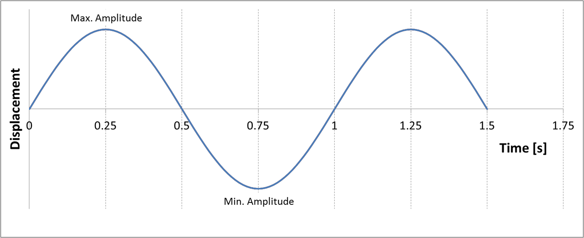
For periodic motion types like Vibration and Pendulum, oscillation is defined by specifying the Amplitude, Frequency, and Initial Phase values for a sine wave.
The Amplitude defines how far the displacement will be, with reference to the original point.
The Frequency defines how many complete cycles will occur per second.
The point at which the motion begins along the sine wave is defined by the Initial Phase value.
To help illustrate how these settings work in practice, let's look at some Initial Phase examples.
An Initial Phase value of zero degrees (default) causes the sine wave to start at the center point of the motion.
For a simple linear oscillation, the frame would move in the following manner:
Frame movement starts at the defined position
Frame moves in the specified direction until it reaches the maximum amplitude
Frame reverses the direction past the starting position and continues until it reaches the minimum amplitude
Frame completes the cycle by reversing direction again back to the original position
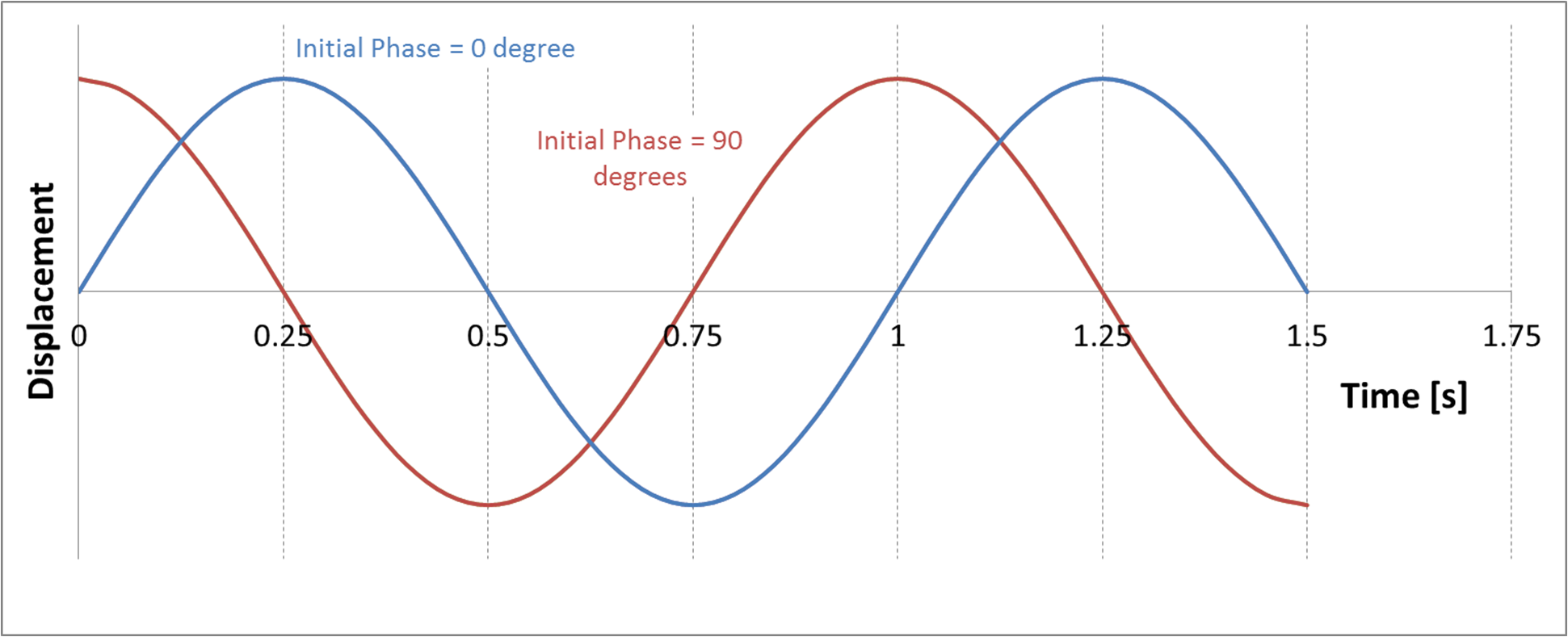
Changing the Initial Phase will change the motion start position. A value of 90 degrees moves the starting point of the sine wave to the maximum amplitude.
In the simple linear oscillation example:
Frame movement starts its motion at the maximum amplitude along the specified direction
Frame reverses the direction, past the starting position and continues until it reaches the minimum amplitude
Frame reverses again to end its cycle at the maximum amplitude position
For this tutorial, we want the vibration motion to have its sine wave start at the center point of the motion (Initial Phase = 0).
We also want a constant oscillation so we will be setting both our Frequency and Amplitude Variation to 0.
Follow the directions to define this motion in a new Motion Frame.
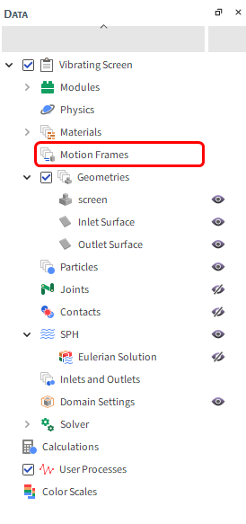
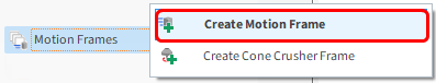
To add a new Motion Frame, from the Data panel, right-click Motion Frames, and then select Create Motion Frame.
To visualize the newly created Frame, click Motion Frames and then in the Data Editors panel, click Preview. A new window will appear showing the geometry and the created Frame.
You can adjust the Frame axes size by changing the Default axes size parameter.
From the Data panel, select the new Frame <01> entry.
From the Data Editors panel, select the Frame tab and then define:
Name: Vibration Motion
Relative Orientation | Angle and Vector
To create a new motion using this Frame, click the green plus button (Add Motion).
Define Type and Direction.
Set Initial Frequency and Initial Amplitude as variables for further optimization analysis (Part C).
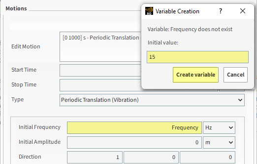
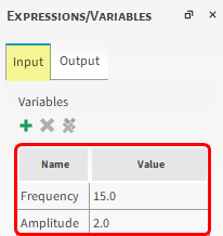
Tip: In Rocky, parameters can be set as variables by typing names instead of numerical values in parameters value fields. In this case, a dialog box for setting up variable Initial Value automatically shows up. Then, you can check (and edit) your variables values on the Expressions/Variables panel through Input tab.
Define Initial Frequency as Frequency, click outside the field, and define Initial Value as 15 Hz
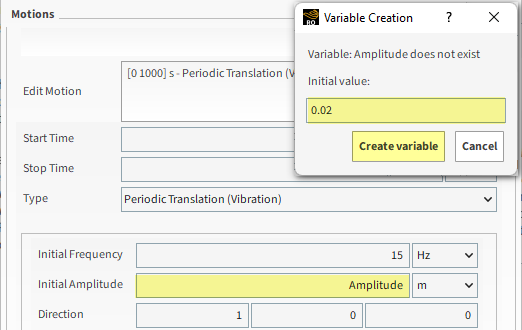
Define Initial Amplitude as Amplitude, with Initial Value of 0.02 m
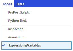
From Menu | Tools, enable the Expressions/Variables panel and check your Variables values in the Input tab
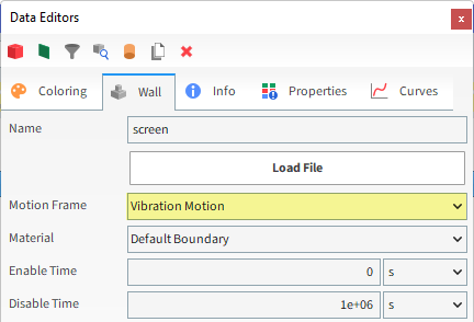
Once the Motion Frame has been created, it must be assigned to the screen.
From the Data panel under Geometries, select screen.
From the Data Editors panel, on the Wall tab, select Vibration Motion from the Motion Frame drop-down list (as shown).
Surfaces can also have Motion Frames assigned to them. We will assign the vibration motion to the Outlet, so that it moves in the same way as the screen.
For this tutorial, since the geometry has a motion with displacement assigned, the movement can be previewed using the Motion Preview window.
The Time toolbar can be used to play the preview. The yellow color of the slider indicates that the simulation has not yet been processed.
For the Materials step, only two materials will be used: one for all the geometry parts (Default Boundary) and another for the particles (Default Particle).
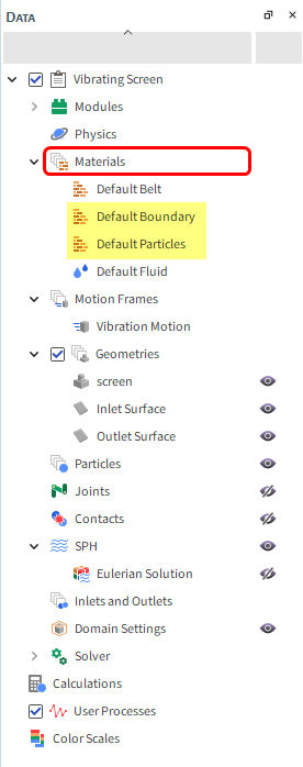
For this tutorial, keep all the values as default for these Materials.
To set the interaction properties, do the following:
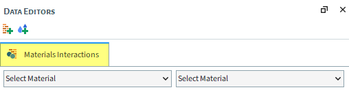
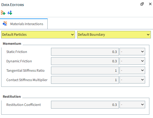
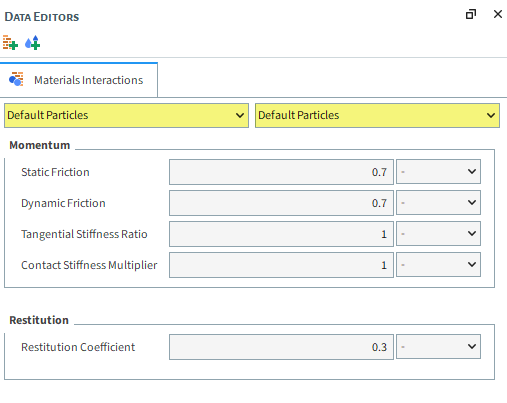
From the Data panel, select Materials. From the Data Editors panel, select the Materials Interactions tab.
From the Data Editors panel, from the left drop-down list, select Default Particles, and from the right drop-down list, select one of its pairs: Default Particles or Default Boundary.
Leave all values as they were set by default, according to the combinations shown below.
For the Particles step, we will create a new sphere-shaped particle group that includes a range of different sizes, and some added rolling resistance.
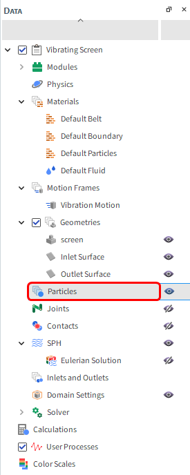
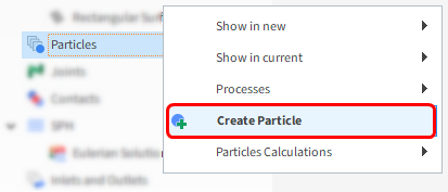
From the Data panel, right-click Particles, and then select Create Particle.
A new particle group is created under Particles.
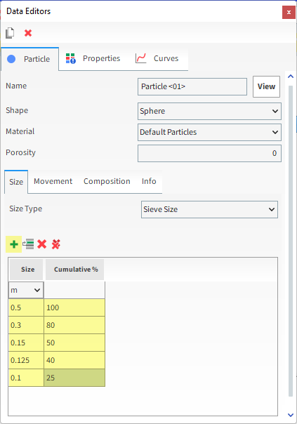
Select the newly created Particle <01> entry to edit its parameters.
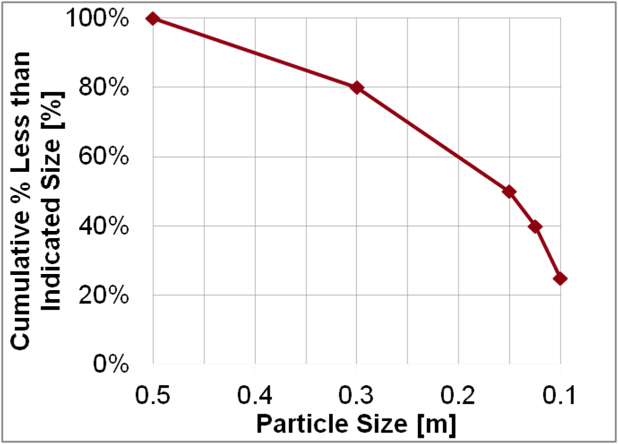
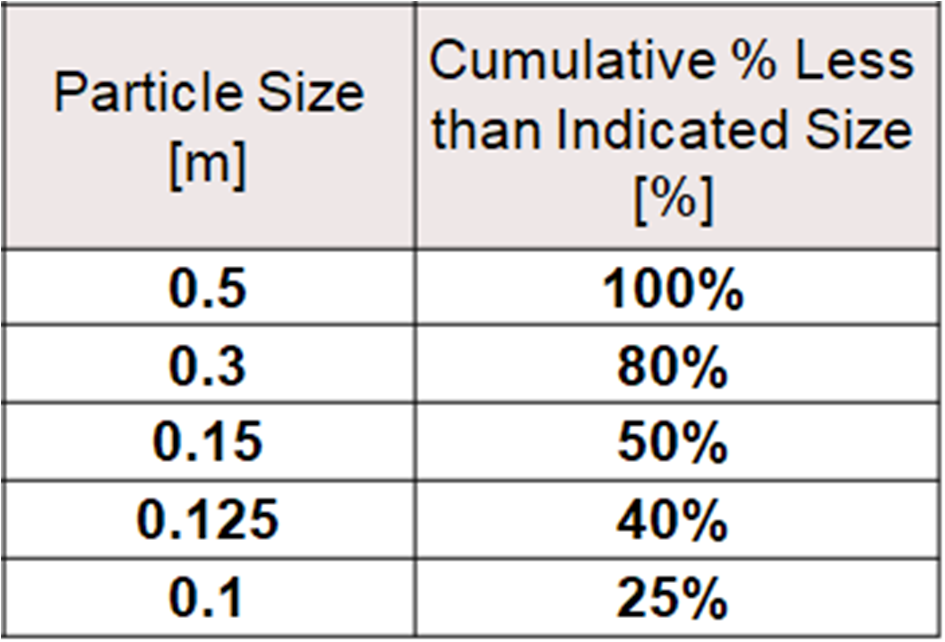
In Rocky, you are able to set a Particle Size Distribution (PSD) for your particles, instead of a single constant value.
Based on sieve analysis, Rocky uses discrete Size ranges and Cumulative % mass of the particles smaller than the specified size.
For this tutorial, the PSD shown below is used, where the smallest particle is 0.1 m, and the largest particle 0.5 m.
From the PSD provided, 50% of the sample mass is below 0.15 m.
To set up the particles for this simulation, follow these steps:
From the Data Editors panel, in the Size sub-tab, click the Add button (green plus) until you have five size definition rows.
For each row, define Size and Cumulative % (as shown).
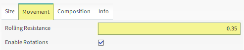
From the Movement sub-tab, define Rolling Resistance (as shown).
To visualize the newly created particle, click View. A new Particles Details window will appear showing the (transparent) particle geometry, its geometric center (yellow dot), and its center of mass (blue dot).
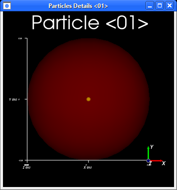
Note: The geometric center and center of mass coincide when the density is uniform throughout the particle.
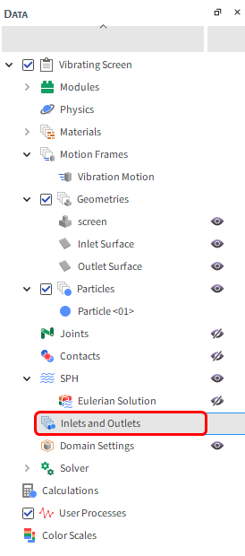
For the Inlets and Outlets step, we will create a Particle Inlet and Outlet, then associate them to the Surfaces we created before.
s
From the Data panel, right-click Inlets and Outlets and then select Create Particle Inlet.
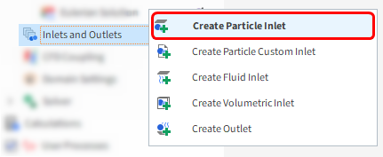
A new entry is created under Inlets and Outlets.
Select the newly created Particle Inlet <01> entry and then from the Data Editors panel, modify the parameters as specified below.
From the main Particle Inlet tab, change Name to Inlet, then select Inlet Surface from the Entry Point drop-down list (as shown).
From the Particles sub-tab, do the following:
Click the green plus button to add a new particle mass flow rate row.
From the Particle column, select the Particle <01> from the drop-down list and then define the Mass Flow Rate in t/h (as shown).
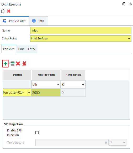
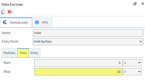
From the Time sub-tab, define the Stop time (as shown).
From the Data panel, right-click Inlets and Outlets and then select Create Outlet.
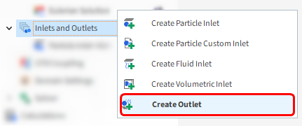
A new entry is created under Inlets and Outlets.
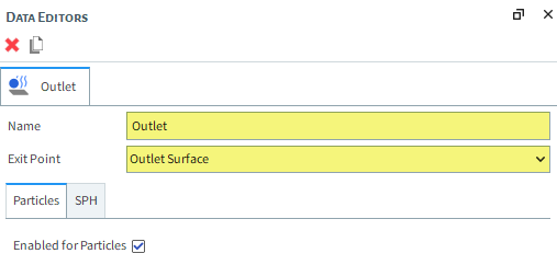
Select the newly created Outlet <01> entry and then from the Data Editors panel, modify the parameters as specified below.
From the main Outlet tab, change Name to Outlet, then select Outlet Surface from the Exit Point drop-down list (as shown).
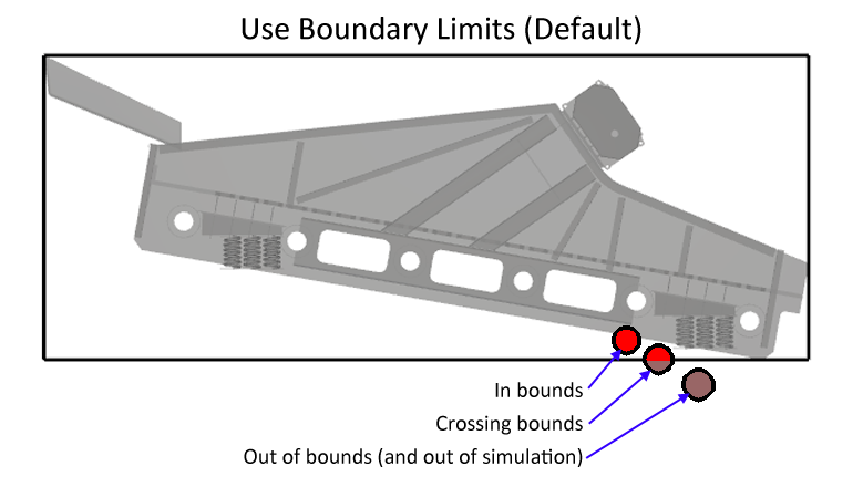
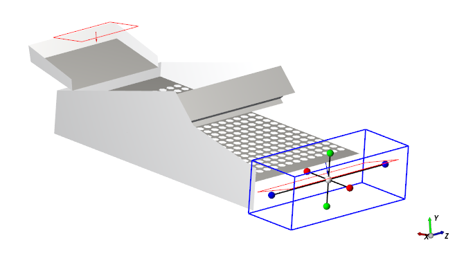
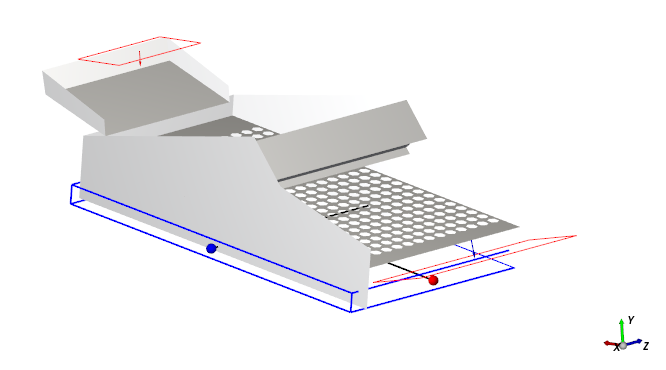
For the Domain Settings step, we will define a custom boundary box that exceeds the limits of our geometry.
Doing this will allow Rocky to compute the particles in the Overflow region.
By default, Rocky automatically creates a domain box based upon the boundary limits of the Geometries.
Any particle that leaves those limits is eliminated from the simulation (as shown).
These default settings would not work for the vibrating screen as the particles would be eliminated before they reached the Overflow area.
To set the boundary limits:
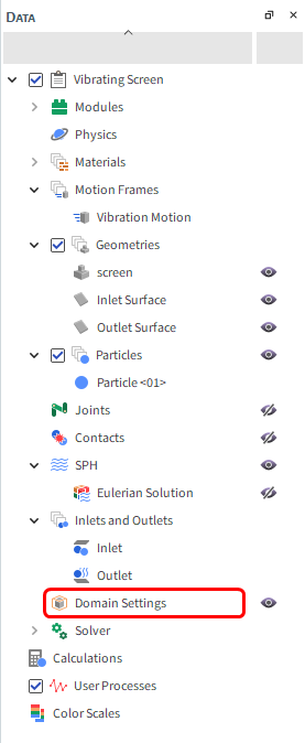
From the Data panel, click Domain Settings.
From the Data Editors panel, clear the Use Boundary Limits checkbox, and then define the Min and Max Values (as shown).

Now let's set up the solver:
From the Data panel, click Solver and then from the Data Editors panel, select the Solver tab.
From the Time sub-tab, define the: Simulation Duration, and Output Settings: Time Interval.
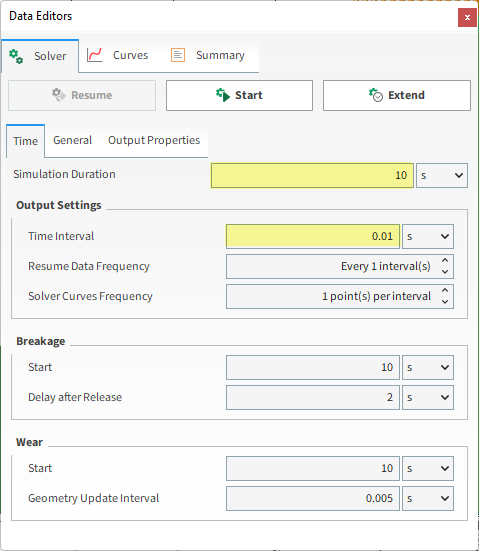
Tip: Saving the outputs more frequently will provide a better view of the vibrations.
From the General sub-tab, set the Simulation Target and the Number of Processors (as shown).

Note: For this tutorial in particular, ensure that you set the Number of Processors to 1. This will ensure the simulation results are consistent for later post-processing.
Click Start.
The Simulation Summary screen appears. This window will disappear on its own, then processing begins.
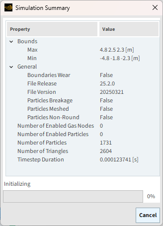
Tip: You can also review this information from the Solver | Summary tab.
To visualize the simulation as it's processing:
From the Window menu, click New 3D View.
Click the Refresh button (or use the Auto Refresh checkbox) to see the results during processing.
Particle states can be viewed in real time as the simulation progresses.
The speed of the simulation depends upon various factors such as:
The particle shape and the number of vertices used to define the shape
Number of contacts in the simulation domain at any time
Number of mesh elements used to define the geometry
Smallest particle size and material stiffness
Frequency of file output
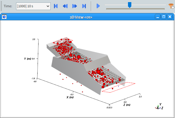
After the simulation is finished processing, it will be clear that the original 10 s Simulation Duration was not long enough for this analysis.
This can be seen by observing that many particles did not leave the domain at the end of the simulation.
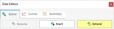
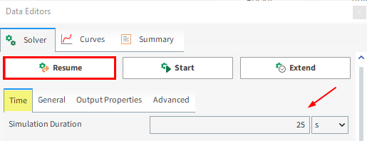
In order to extend the simulation without losing the results, from the Solver tab, click Extend.
From the Extend Simulation window, define the Extend by value (as shown), and then click OK.
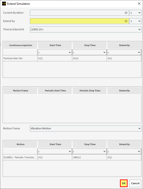
On the Data Editors panel, from the Solver | Time tab, note that the Simulation Duration has been updated to show the new total time of 25 s.
Click Resume to continue processing.
The Simulation Summary screen appears again. This will disappear on its own, then processing resumes.

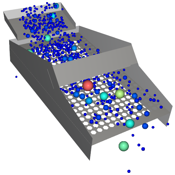
At the end of the newly extended simulation (25 s), no particles are left on the screen (as shown).
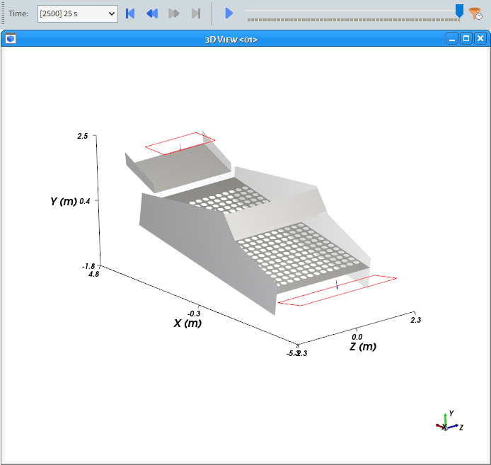
This means that we are ready to analyze the results of the simulation.
This completes Part A of this tutorial.
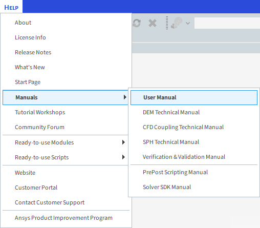
For further information on any topic presented, we suggest searching the User Manual, which provides in-depth descriptions of the tools and parameters.
To access this manual, from the main Toolbar click Help, point to Manuals, and then click User Manual.
Rocky was used to set up and process a vibrating screen simulation.
During this tutorial, it was possible to:
Use Motion Frames to set up a vibration motion
Define a particle size distribution (PSD)
Set custom domain limits
Extend the simulation duration
What's Next? If you completed this tutorial successfully, then you are ready to move on to Part B and post-process this project.
The main purpose of this tutorial is to learn how to analyze the screening efficiency of a vibrating screen using User Processes, custom Curves, and Time Plot functions. We will continue from where we left off in Part A.
You will learn how to:
Employ User Processes to define different analysis areas
Create a custom Curve
Create a Time Plot table view and add custom functions
View and customize a Histogram
And you will use these features:
User Processes, including:
Cube
Property
Particles Time Selection
Curves
Time Plot
Histogram
This tutorial assumes that you are already familiar with the Rocky user interface (UI) and with the project workflow.
If this is not the case, please refer to Tutorial 01 – Transfer Chute for a basic introduction about Rocky usage before beginning this tutorial.
If you completed Part A of this tutorial, ensure that project is open in Rocky. (Part B will continue from where Part A left off.)
If you did not complete the project from Part A, do all of the following:
Download the
dem_tut03_files.zipfile here .Unzip
dem_tut03_files.zipto your working directory.Open Rocky 2025 R2.
From the Rocky program, click the Open Project button, find the tutorial_03_input_files folder, then from the tutorial_03_A_pre-processing folder, open the tutorial_03_A_pre-processing.rocky file.
From the Rocky program, click the Open Project button, find the dem_tut03_files folder, then from the tutorial_03_A_pre-processing folder, open the tutorial_03_A_pre-processing.rocky file.
Process the simulation. (From the Simulation toolbar, click the Start button.)
Once the simulation is finished processing, you are ready to start Part B.
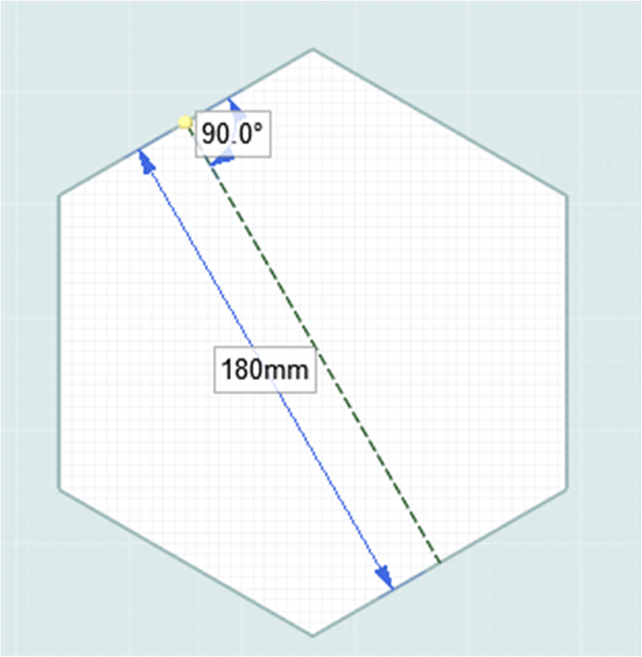
In this tutorial, the Screen Efficiency will be calculated. As the sieve size of the screen mesh is 180 mm:
Particles with diameter >180 mm will be considered Oversized Particles
Particles with diameter <180 mm will be considered Undersized Particles
Screen Efficiency based on Oversized:

Screen Efficiency based on Undersized:

Total Screen Efficiency:

To calculate the necessary variables, the particles must be sampled using the following User Processes:
Cubes: One to account for the particles that went through the screen (Underflow) and a second to account for the particles that did not go through the screen (Overflow).
Filters: Three, to filter the particles by size in separate locations.
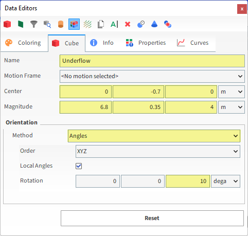
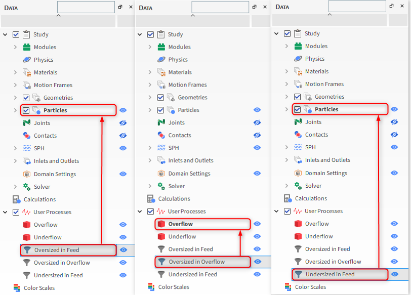
The first User Process will be a Cube. To create it, follow these steps:
From the Data panel, right-click Particles, point to Processes, and then select Cube.
From the Data Editors panel, ensure that the Cube tab is selected and then change the Name to Underflow and use the values shown in the image below to define the Center, Magnitude, Orientation | Method and Rotation.
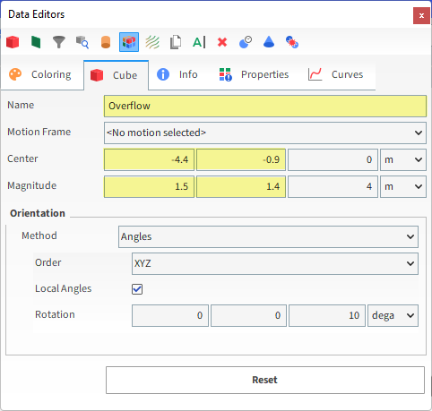
To create the second Cube, do the following:
From the Data panel, under User Processes right-click the Underflow User Process, and then select Duplicate.
A new Underflow <01> entry appears with the same values you entered earlier.
For this new Cube entry, change the Name to Overflow and use the values shown in the image for Center and Magnitude (as shown).
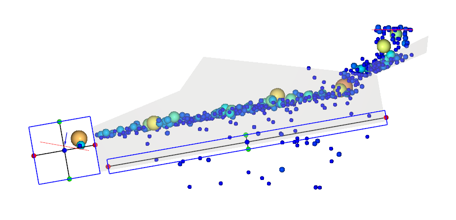
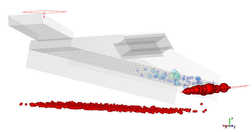
At this point in the tutorial, when you select one of the Cubes in the Data panel, the 3D View should show the cubes in blue.
To finish the sample creation, both the particles that are fed and the ones that end up in the Overflow cube must be divided based upon the size. (This is not necessary for particles in the Undersized cube since all sieved particles are below 180 mm.)
To create these size filters, the Filter User Process will be used with the following three processes:
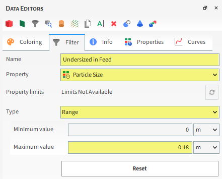
Undersized in Feed: Created from Particles with a Particle Size filter smaller than 180 mm.
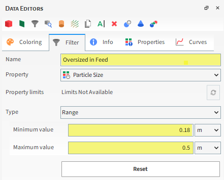
Oversized in Feed: Created from Particles with a Particle Size filter larger than 180 mm.
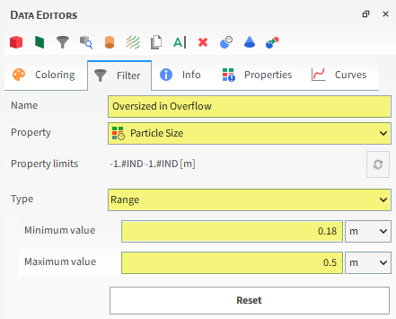
Oversized in Overflow: Created from Overflow with a Particle Size filter larger than 180 mm.
To set up the Filter User Processes:
Right-click Particles, point to Processes, and then select Filter.
A new Filter <01> entry is created beneath Underflow.
For this new entry, change the Name to Undersized in Feed and use the values shown in the image for Property, Type and Maximum value.
For the second Filter, right-click Undersized in Feed in Data panel, and then select Duplicate. A new Undersized in Feed <01> entry appears with the same values you set earlier.
For this new process, change the Name to Oversized in Feed and use the values shown in the image for Minimum value and Maximum value.
For the third Filter, right-click Overflow (Cube), point to Processes, and then select Filter. A new Filter <01> entry appears.
For this one, change the Name to Oversized in Overflow and use the values shown in the image for Filter, Type, Minimum value, and Maximum value.
Please take a moment to verify that each of the three Filter User Processes matches the settings in the images below.
To correctly evaluate the screen efficiency, all the mass that passed through the screen and the mass that remained above the screen need to be accounted for.
Rocky has two different ways to include the particles that crossed the boundary limits:
Custom Curves: Curves can be customized in Rocky to include time functions and advanced curves based upon multiple Properties.
Particles Time Selection: A time filter can be used to include all the particles that were present in a specific sample for a given time frame.
For this tutorial, the Custom Curves will be used to calculate the screen efficiency and the Particles Time Selection will be used to compare the PSD in the Feed and in the Overflow areas.
A Custom Curve created for either the Particles or Geometries will be available for all the associated User Processes within this project.
There are two ways to save Custom Curves and Custom Properties, within the project or locally. By choosing to Save in Project, the custom Curve or Property is saved within that specific Rocky Project and is only available in said project. By choosing to Save Locally, the custom Curve or Property is not restricted to the Rocky Project it was created in, and extends to any other projects created on your computer.
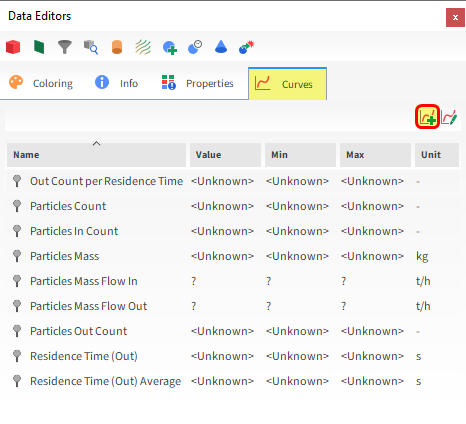
To create a custom curve for this tutorial:
From the Data panel, select Particles.
From the Data Editors panel, on the Curves tab, select the Add new custom curve icon (as shown).
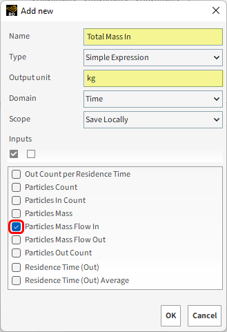
From the Add new window that appears, enter the Name and Output unit (as shown).
Under Inputs, you must select all the curves that will be used to define the new Custom Curve. In this case, select Particles Mass Flow In, which accounts the mass flow that enters a region at a given time.
Click OK.
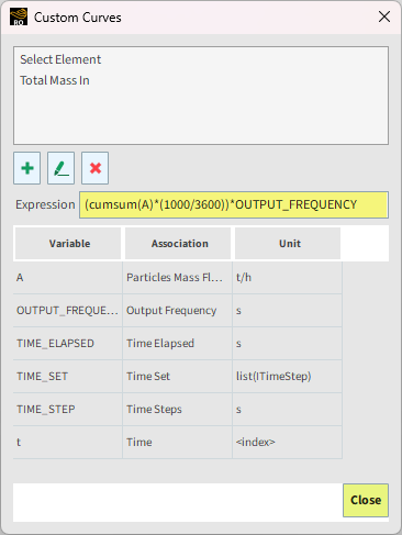
The Custom Curves window appears with the new Curve selected.
The function we will use for this Total Mass In curve is the cumsum(), which returns the cumulative sum of the selected variable over time.
The available Variables are listed below Expression, along with their Association and Unit.
Continue defining the Curve as follows:
In the Expression field, enter the shown expression to calculate the sum of the mass of particles that got into the domain in the desired unit (kg).
Click OK.
The new Total Mass In (Custom) Curve is now available in the Curves tab, under custom.
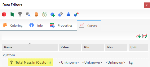
Tip: If your Curve does not appear in the Curves tab immediately, select another item in the Data panel and then come back to this tab to refresh it.
To visualize the curves, we'll now create a Time Plot:
From the Window menu, click New Time Plot (or click Ctrl + T)
From the Data panel, under User Processes, select Underflow.
From the Data Editors panel, on the Curves tab, drag and drop the Total Mass In (Custom) curve over the grid.
Note: Due to the calculations involved, it may take a few minutes for the data to display.
Tip: To ensure that the curves appear in the right order, it is best to wait for one curve to finish processing before adding the next one.
One-by-one, also drag-and-drop the Total Mass In (Custom) curve from the Curves tab for each of the following User Processes:
Note: It is important to follow this order.
Oversized in Overflow
Undersized in Feed
Oversized in Feed
The Time Plot should now show four data sets (as shown).
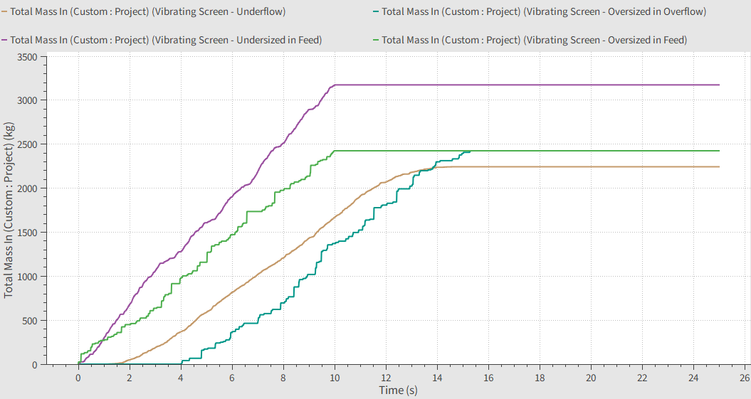
Note: The order that you add the curves affects the column order of the Table tab (shown below).
For further optimization analysis (Part C), select the Output tab of Expressions/Variables panel (enabled in Part A), and drag and drop the same four curves (Total Mass In (Custom) for Underflow, Oversized in Overflow, Undersized in Feed and Oversized in Feed User Processes) into the Output Variables field.
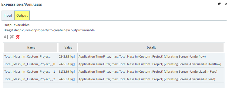
Note that for every Output Variable, the default settings consider the maximum values for the curves, that match the last output values.
One by one, Edit the Output Variables (click
 ) and define the Name for each one accordingly:
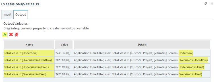
Tip: The steps 5 to 7 allow and facilitate optimization analysis using optiSLang (Part C).
Rocky allows you to use a Table view to create Formulas in the Time Plot.
To switch to this view, from the top left of the Time Plot window, click the Table tab.
Please take a moment to ensure that data in the Element row matches the column order of the screenshot. The three efficiencies will be calculated based upon this order.
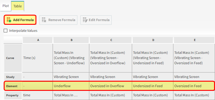
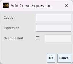
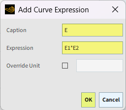
To define each formula, click Add Formula, and then from the Add Expression window, fill in the Curve Caption and Curve Expression values as shown below.
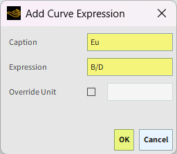
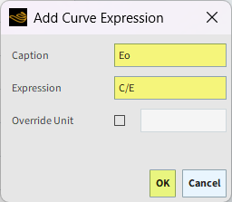
In the Add Expression window, define all three equations as shown below. Keep in mind that the column order matters, so ensure the EU and EO are correctly defined in the order specified.


From the Table tab, it is possible to evaluate the screening efficiency by viewing the data at the very end of the table:
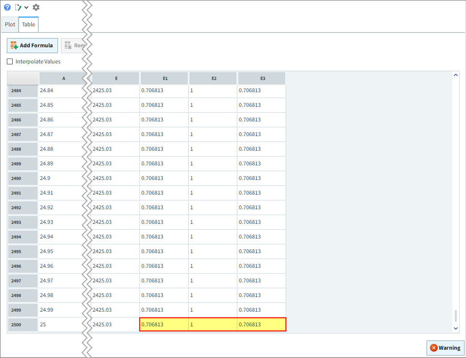
EU = 0.706813
EO = 1
E = EU * EO = 0.706813
Note: The values you end up with in your project may vary slightly from the ones shown in this Tutorial.
Achieving 1 (max value) on the undersized efficiency (Eu) means that every undersized particle inputted went through the sieve as desired.
In this case, EU = 0.706813, which means that not all of the Undersized particles passed through the screen. Looking at the 3D View, we can see that many smaller particles exited with the bigger particles in the Overflow area.
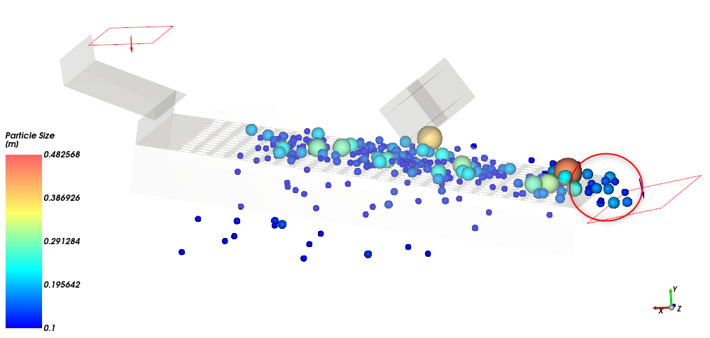
An adjustment in vibration may improve the screening efficiency, as may a screen redesign.
Achieving 1 (max value) on the oversized efficiency (Eo) means that all the oversized particles inputted moved over the Screen and into the Overflow area as desired (this case).
The Particles Time Selection is a powerful tool to sample the particles based upon the simulation time.
The first Particles Time Selection will be created for the whole domain, so this should be created for the Particles entity.
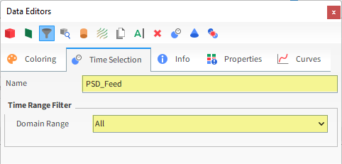
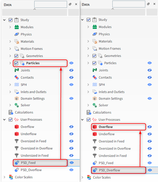
From the Data panel, right-click Particles, point to Processes, and then select Particles Time Selection. A new Particles Time Selection <01> entity appears.
From the Data Editors panel, select the Time Selection tab.
Change the Name to PSD_Feed and to include the entire time range, from the Domain Range drop-down list, select All.
Repeat the same procedure for the Overflow Cube.
From the Data panel, right-click Overflow, point to Processes, and then select Particles Time Selection.
From the Data Editors panel, select the Time Selection tab, and then change the Name to PSD_Overflow.
From the Domain Range drop-down list, select All (as shown).
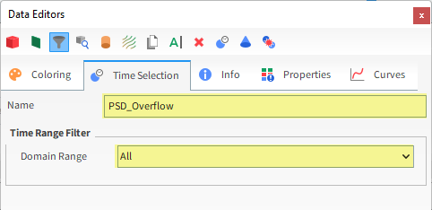
Please take a moment to verify that both Particles Time Selections match the settings in the images.
Histograms are used to create bar plots showing Properties values and their distribution among the selected samples in a given Output.
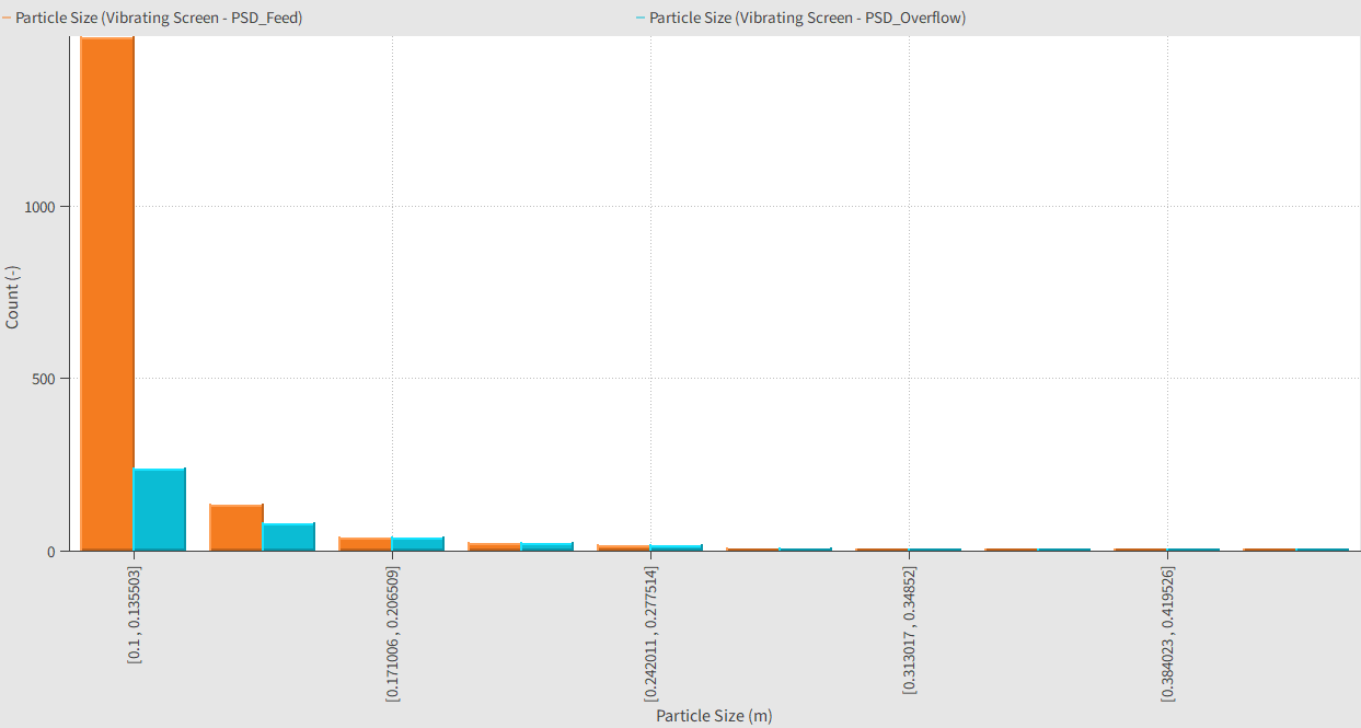
In this tutorial we will use a Histogram to compare the PSD of the Feed with the PSD of the Overflow.
To create a Histogram, from the Window menu, select New Histogram (or use the shortcut Ctrl+H).
From the Data panel, select PSD_Feed.
From the Data Editors panel, select the Properties tab, and then drag and drop Particle Size onto the Histogram window.
Repeat this process to include on the Histogram the Particle Size property for the PSD_Overflow process.
The results are shown below.
The default settings provide a plot that is difficult to analyze. To improve the analysis, click the Configure histogram icon at the top left of the Histogram window.
The Configure Histogram window appears.
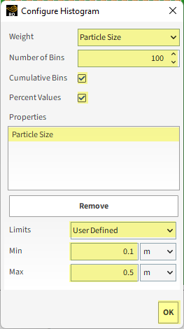
The cumulative PSD distribution plot is linear with the mass plotted between the specified sizes.
To reproduce this plot, select the distribution Weight, increase the Number of Bins, and activate both Cumulative Bins and Percent Values (as shown).
The axes limits can be specified by selecting Particle Size (under Properties) and then changing the Limits to User Defined (as shown).
Specify the Min and Max values (as shown), and then click OK.
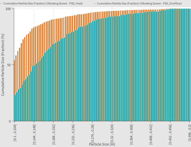
Compared to the default settings, the reconfigured Histogram better illustrates how different the PSDs are before and after the sieve.
The PSD from Feed (green bars) shows a higher percentage of mass in the smaller sizes.
It can also be seen that particles smaller than the screen aperture have left the screen from the Overflow area.
This completes Part B of this tutorial.
For further information on any topic presented, we suggest searching the User Manual, which provides in-depth descriptions of the tools and parameters.
To access this option, from the main Toolbar click Help, point to Manuals, and then click the User Manual option.
Rocky was used to analyze the screening efficiency of the vibrating screen simulation we created in Part A.
During this tutorial, it was possible to:
Use the Cube, Filter, and Particles Time Selection User Processes to calculate particle screening efficiencies
Create a custom Curve
Plot data in a Time Plot and use the Table view to add custom functions
Use a Histogram to plot and compare the efficiency results
What's Next? If you completed this tutorial successfully, then you are ready to move on to Part C and optimize this project with optiSLang.
The main purpose of this tutorial is to learn how to make optimization analysis via optiSLang for the screening efficiency of a vibrating screen. We will continue from where we left off in Part B.
You will learn how to:
Set up an optiSLang project for optimization of a Rocky project
Define criteria variables
Set parameter ranges
And you will use this feature:
optiSLang Optimization wizard
To complete this tutorial, you are required to have on your machine both of the following:
(1) A license of Ansys optiSLang 2025 R2.
(2) A license of Rocky 2025 R2 or later.
(3) Tutorial 03 project folder with Part A and B data already processed.
Important: If you skipped Part A and used the already set up tutorial_03_A_pre-processing.rocky project file for going through Part B, you will have to follow step 7 from Section 3.1.15 (Part A) in order to create Rocky Inputs for optimization analyses. If you went through Part A step by step, you are ready to start Part C.
Important: This tutorial assumes that you are already familiar with the following programs and resources:
The Ansys optiSLang platform.
Rocky user interface (UI) and project workflow.
If this is not the case, please refer to Tutorial 01 – Transfer Chute for a basic introduction about Rocky usage before beginning this tutorial.
When running any analysis in optiSLang, some files are created inside the project folder. As a good practice, you might have a folder containing only your Tutorial 03 Rocky files (.rocky file and .rocky.files folder) as your project directory to start with the optiSLang project creation.
To begin the steps for the optiSLang project creation, do the following:
Open optiSLang 2025 R2.
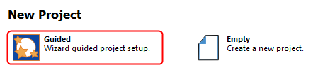
From the optiSLang New Project field, select Guided to start the project setup.
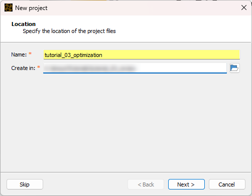
From the New Project window that appears, define the File name as tutorial_03_optimization, select your project directory, then click Next. Review your project information and click Finish.
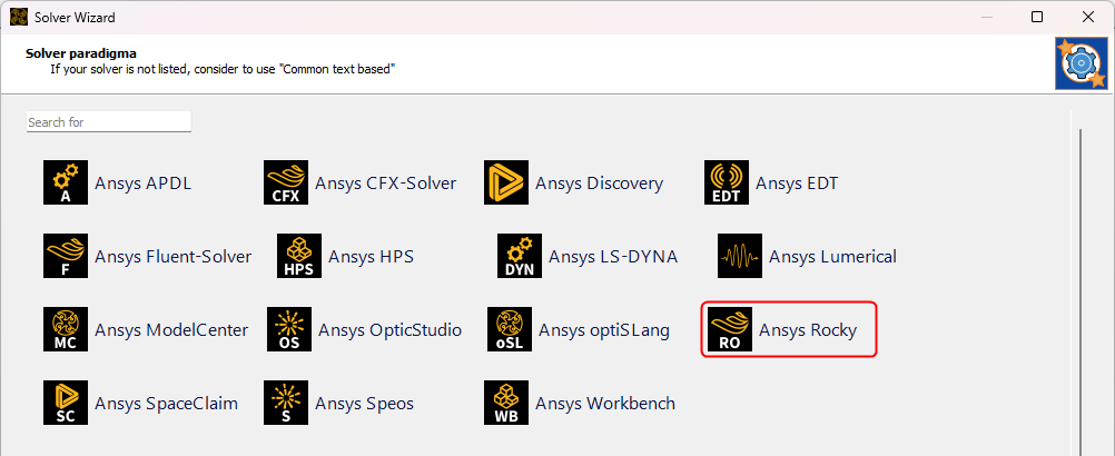
From the Solver Wizard window, select Ansys Rocky.
From the Select project file dialog, go to your project directory and select your Tutorial 03 project file.
After selecting the Rocky project, a new window will show up to select a python script (automatically created by optiSLang) to export Rocky results.
From the Choose Rocky script to export results., select the brand new export_rocky_outputs.py that is in your project directory and click Open.
Rocky opens with the selected project loaded and will save a copy without results, asking if you want to delete the results.
Click Yes to complete the Wizard setup (project closes).
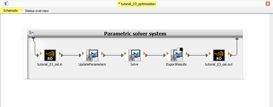
Your project Schematic in optiSLang should now look like the image:
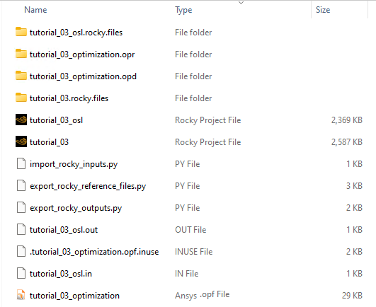
And your project directory should look similar to the image below.
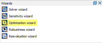
Many analyses can be done in optiSLang through its Wizards, which guide the user in order to facilitate the project setup. In this tutorial, we are going to use the Optimization wizard to start our Rocky project optimization setup.
Tip: You can access the Wizards panel through the optiSLang user interface, in the top right corner of the window.
Follow the steps below to configure optimization settings.
From the Wizards panel, drag and drop the Optimization wizard onto the Parametric solver system box in the project Schematic.
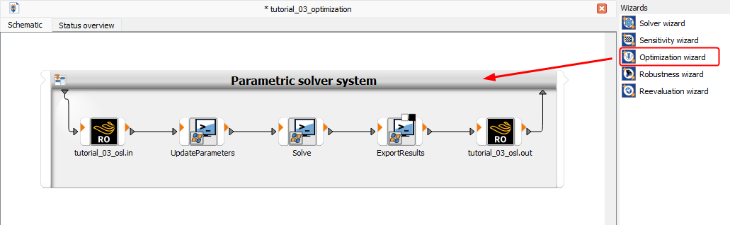
The Optimization Wizard dialog box shows up to Parametrize Inputs.
Note: optiSLang loads Rocky inputs that we defined as variables in Part A of this tutorial.
Set the Range for both parameters according to the following image and click Next >:
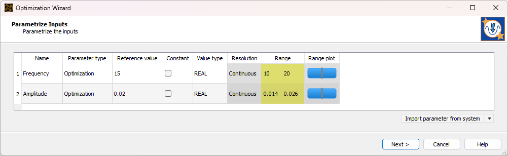
Note that optiSLang considers the inputs limit values to define the design points that will be processed posteriorly in Rocky. In this case, Frequency will be varied from 10 Hz to 20 Hz, and Amplitude will vary from 0.014 m to 0.026 m, for example.
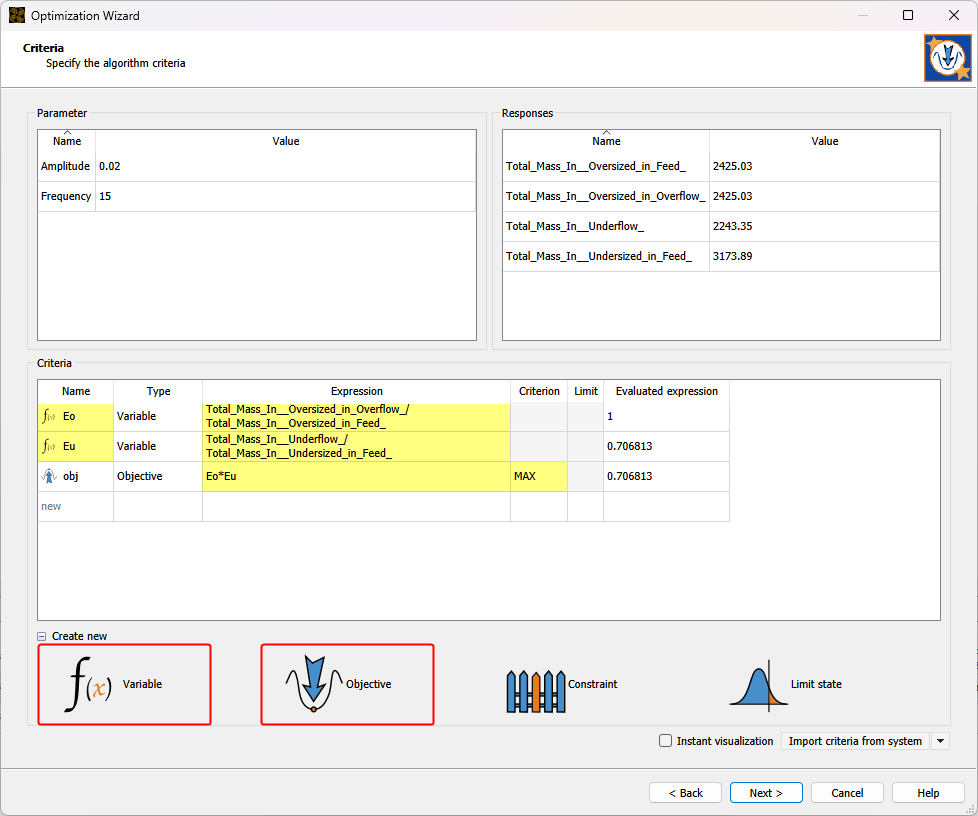
In the Criteria step of the wizard, you can define new variables using Rocky inputs and outputs, and even performing mathematical operations between them. In this step you can also define an Objective to optimize the response you want from your Rocky simulation.
For this step, we want to define the screen efficiency (defined in Rocky in Part B) as a Variable in optiSLang and set an Objective for it. For this, follow the steps and the image shown.
On the Criteria | Create new field, click two times in the Variable button and one time in Objective button.
Define the Name and Expression for each new Variable.
Note: This process is similar to the one done in the Table of the Time Plot in Rocky, in Part B.
Define the Expression and Criterion for the objective in order to maximize the screen efficiency.
Click Next > to continue setting your optimization project.
In the Optimization method step, you can set parameters to define how optiSLang will process the simulations with the evaluated design points. To get specific information about these calculations, check the optiSLang documentation.
For this tutorial, we will define the maximum number of simulations to be processed and let the other parameters as default.
Define the Maximum number of design evaluations and click Next >.
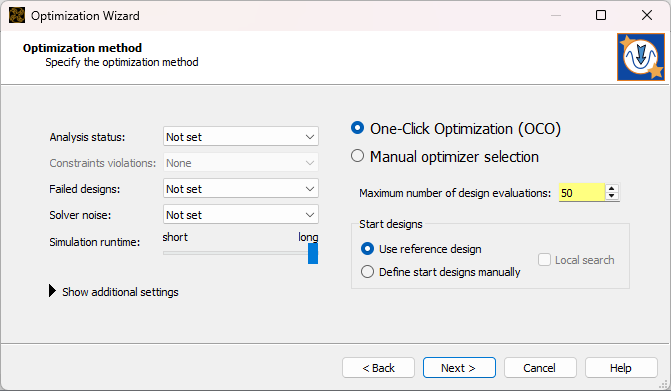
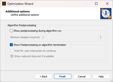
On Additional options, you can choose to visualize the postprocessing during the optimization processing or when it finishes. For this tutorial purposes, we only need to visualize it on termination, so you might let the settings as default and click Finish.
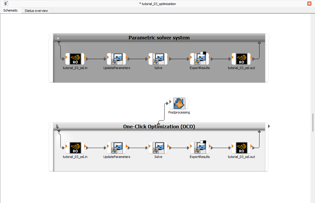
Your project Schematic should now look similar to the image below.
After passing through every section of the wizard, we are ready to run the optimization case.
In the top left corner of the optiSLang user interface, click the Run button
 to run the optimization analysis.
Note: For each design point evaluated, Rocky opens to set the Amplitude and Frequency values and process the simulation.
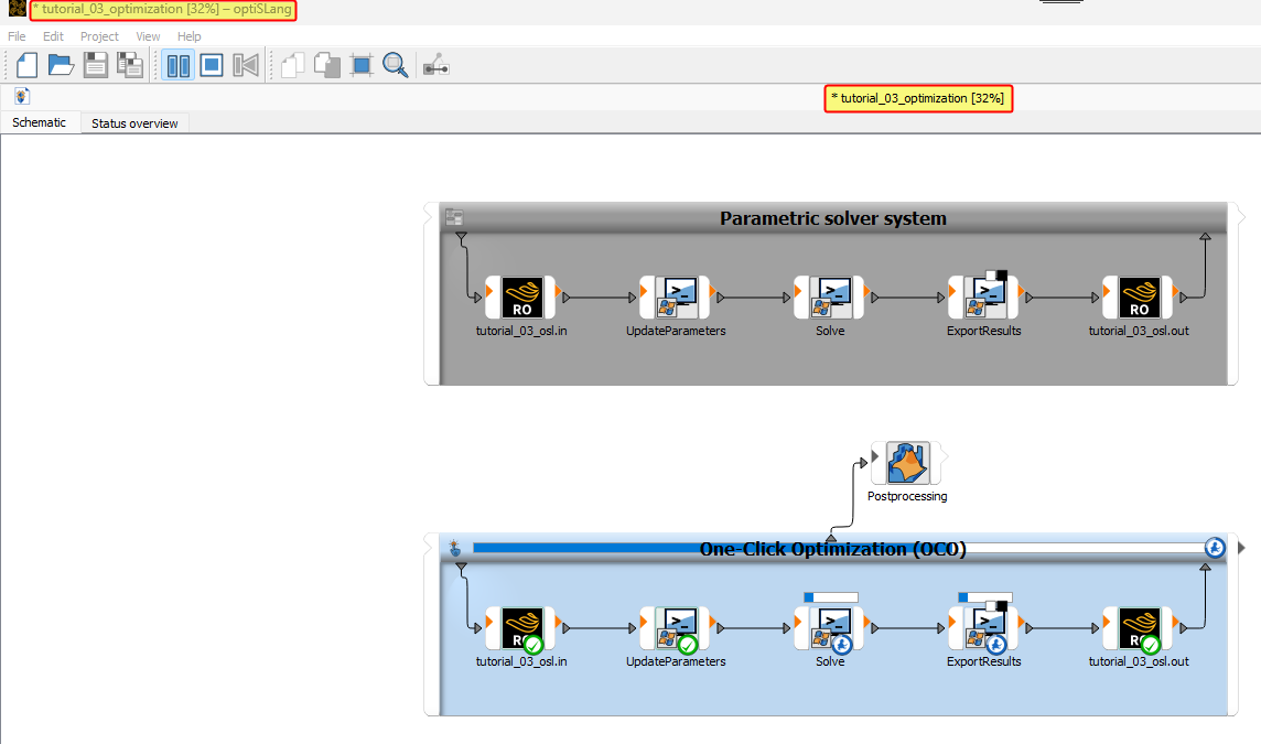
You can check the progress of your analysis in optiSLang user interface.
When the algorithm finishes running the analysis, a post-processing window opens automatically. If you reopen your project, you can access the same data by double-clicking Postprocessing in the project Schematic.
By default, optiSLang shows four post-processing result panels (as shown): History, Response values, Design parameter and Criteria data.
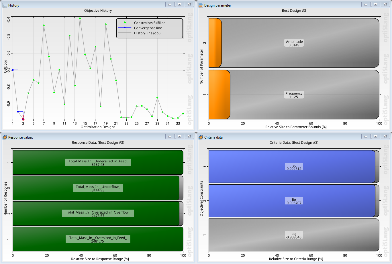
Each one of these panels will be detailed below.
History
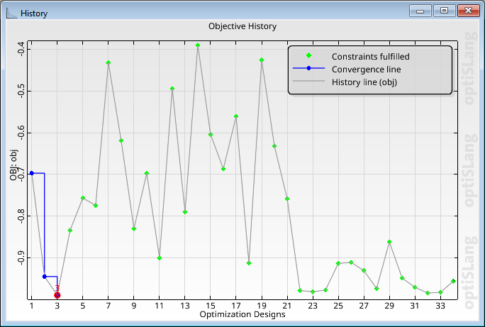
This panel shows the evolution of the objective through different combinations of Amplitude and Frequency (design points). It also indicates in which design point the solution obtains the best results.
Note: You can click on each (design) point in the plot and see its results in the other panels. By default, the selected one is the best for optimization purposes.
Response values
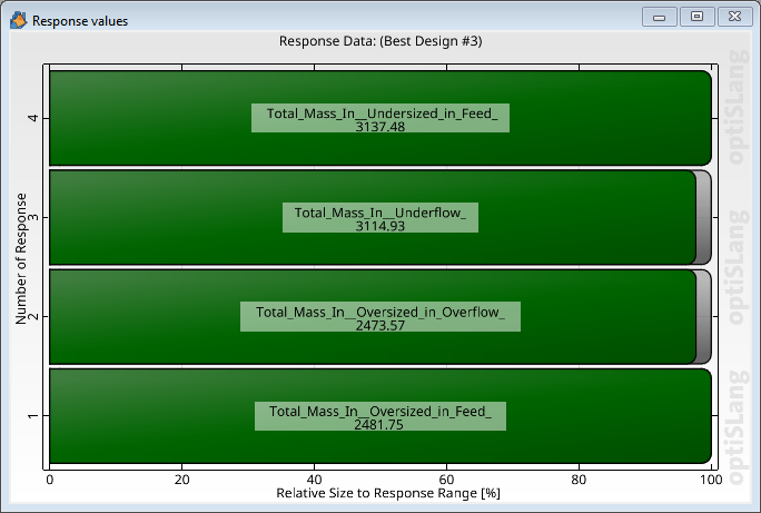
This panel shows the resulting values of each Rocky Output Variable for the selected design point in the first panel.
Design parameter
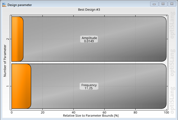
This panel shows the values of Rocky Input Variables (Amplitude and Frequecy) for the selected design point.
Criteria data
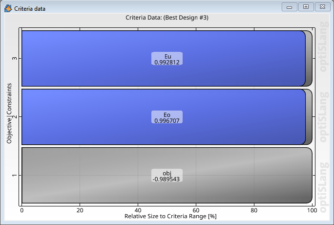
This panel shows the numerical values of the variables defined in the Criteria step of the Optimization wizard for the selected design point.
Note: The optimization project brought an improvement in screen efficiency if compared to what was observed in Part B, from 0.70 to 0.98.
Note: Your results may vary slightly from the ones presented in this tutorial.
This completes Part C of this tutorial.
For further information on any topic presented, we suggest completing the optiSLang courses available at Ansys Innovation Space (AIS) and Ansys Learning Hub (ALH).
Ansys optiSLang was used to optimize the screening efficiency of the vibrating screen simulation we created in Part A and post-processed in Part B.
During this tutorial, it was possible to:
Create a coupled project using Rocky and optiSLang
Use the Optimization wizard
Parametrize and define range of analysis for Rocky variables
Define and analyze an Objective to guide optimization process
What's Next? If you completed this tutorial successfully, then you are ready to move on to next tutorial.