


(Part A) Set up and run a SAOR test case using a cylinder and tray.
(Part B) Calculate the resulting SAOR using two methods: manually using Cross Plots and automatically using a Python script.
(Part C) Study how the SAOR behaves with different particle-to-particle static and dynamic friction values by running multiple cases in the Rocky Scheduler.
The purpose of this tutorial is to run a Static Angle of Repose (SAOR) test case with different material and interaction parameters in order to validate the DEM coefficients for future simulations.
You will learn how to:
Set up an adhesion model
Change material values
Inject particles by Volumetric Inlet
And you will use these features:
Materials and Materials Interactions
Volumetric Inlet
Important: Even though this tutorial involves running only one SAOR test, other simulations must be done in order to calibrate the particle model in full.
This tutorial assumes that you are already familiar with the Rocky user interface (UI) and with the project workflow.
If this is not the case, please refer to Tutorial 01 - Transfer Chute for a basic introduction about Rocky usage before beginning this tutorial.
This tutorial uses SI Units as default units.
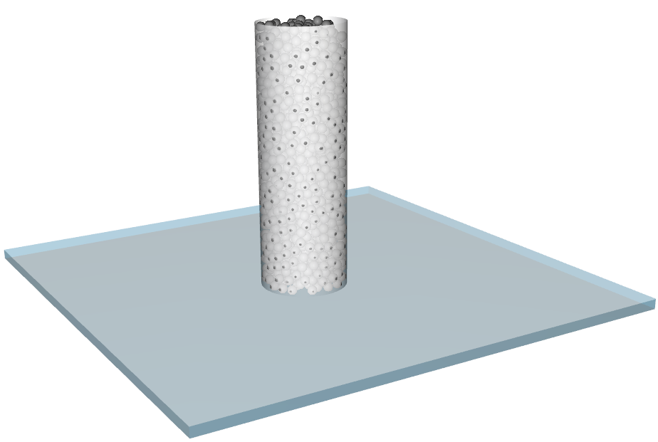
The geometry in this tutorial is composed of:
(1) Container cylinder
(2) Upper Tray
In the tutorial directory each .stl file can be found.
To start the tutorial, let's create a new project:
Download the
dem_tut02_files.zipfile here .Unzip
dem_tut02_files.zipto your working directory.Open Rocky 2025 R2. (Look for Rocky 2025 R2 in the Program Menu or use the desktop shortcut.)
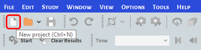
From the Rocky program, click the New Project button, or from the File menu, click New Project (Ctrl+N).
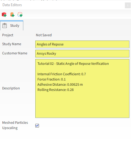
The Study entity covers the first step of the simulation setup. The purpose is to define any useful information for the project.
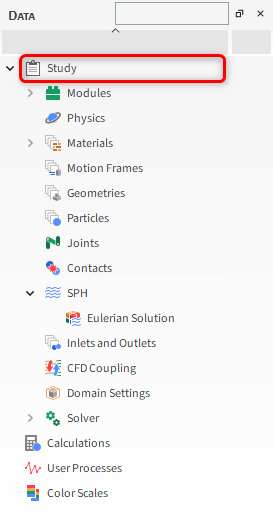
From the Data panel, click Study.
From the Data Editors panel, enter the project information.
For the Physics step, we will be adding a rolling resistance model and an adhesive force and will be lowering the softening factor to reduce the simulation time.
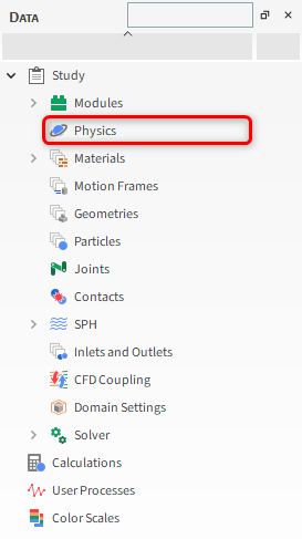
From the Data panel, select Physics.
From the Data Editors panel, select the Momentum sub-tab, and then define all of the following:
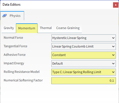
Important: Lowering the softening factor may cause excessive overlaps between particles and between particles and boundaries.
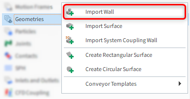
For the Geometries step, we will import geometry files in .stl format.
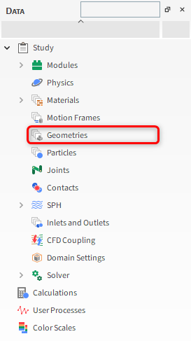
From the Data panel, right-click Geometries and then click Import Wall.
From the Select file to import dialog, navigate to the dem_tut02_files folder that you previously downloaded, find the geometry folder, and then while pressing either the Ctrl or Shift key, multi-select all of the following files, and then click Open:
Container_Cylinder.stl
Upper_Tray.stl
(Save your project now if you have not already done so.)
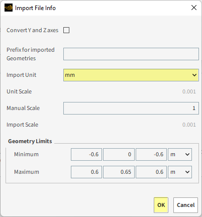
From the Import File Info dialog, select "mm" as Import Unit, ensure that the option Convert Y and Z axes is cleared (unchecked), and then click OK (as shown).
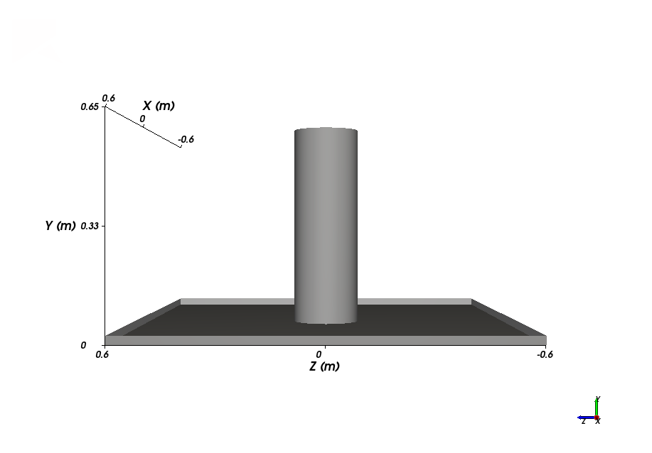
After the geometry is imported, you can view the results in a 3D View window:
Drag and drop the Geometries entity from the Data panel onto the Workspace. A new 3D View window appears showing the geometries that you imported.
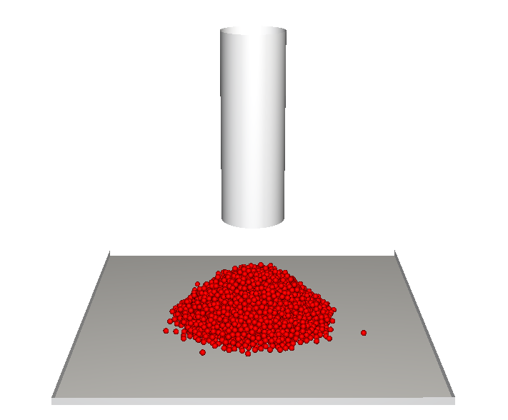
In this tutorial, after the cylinder container has been filled with particles, it slowly moves up and away from the tray, which allows the particles to spread out and form a pile.

To compute the boundary movement, a motion frame of the type Translation needs to be selected.
After selecting Translation, the following options will be available:
Fixed Velocity: Constant velocity will be defined in the local coordinates.
Initial and Final Velocity: The velocity at the Start Time and at the Stop Time will be defined in the local coordinates and the Acceleration will be calculated.
Initial Velocity and Acceleration: With the Stop Time fixed, the velocity at the Start Time and the Acceleration will be defined in the local coordinates and the velocity at the Final Velocity will be calculated.
Note: The following procedures include step-by-step directions on how to create the motion frame.
To add a new Motion Frame, do the following:
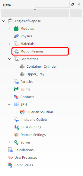
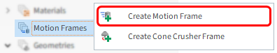
From the Data panel, right-click Motion Frames, and then select Create Motion Frame.
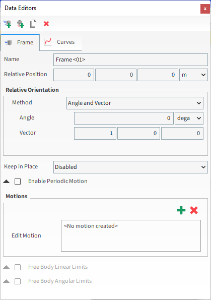
From the Data panel, under Motion Frames, select the newly added Frame <01> entry.
From the Data Editors panel, on the Frame tab, define the parameters as shown on the next section.
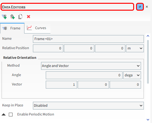
At this point, you may not be able to see the entire Data Editors panel by default (as shown).
Tip: To display more of the panel, you can drag and drop it by its header, double click it or click the blue button to make it float. This can facilitate the visualization of the fields.
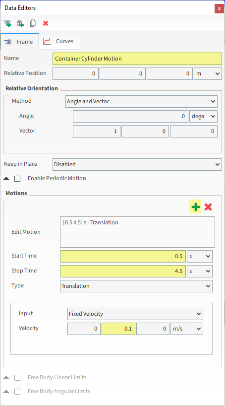
Define the Name: Container Cylinder Motion
To create a new motion for this Frame, do the following:
Click the green plus button (Add motion).
Set the Type as Translation motion (default).
In order to settle the particles inside the cylinder before it rises, we want this motion to have a slight delay. So define the Start Time, Stop Time and Velocity.
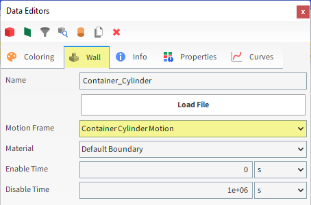
Once the Motion Frame has been created, it can be assigned to the Cylinder geometry:
From the Data panel, under Geometries, select Container_Cylinder.
From the Data Editors panel, on the Wall tab, from the Motion Frame drop-down list, select Container Cylinder Motion (as shown).
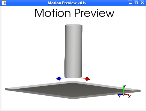
For this tutorial, since the geometry has a motion with displacement assigned, the movement can be previewed using the Motion Preview window.
From the Data panel, select Motion Frames.
From the Data Editors panel, click Preview (as shown). A new window will appear showing the geometry and the created Frame.
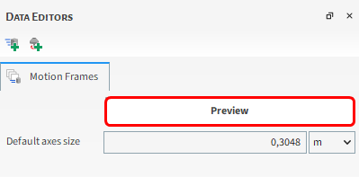
Tip: You can define the axes size for better visualization with the Default axes size parameter.
The Time toolbar can be used to play the preview. The yellow color of the slider indicates that the simulation has not yet been processed.

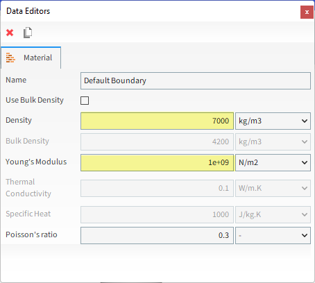
For the Materials step, only two materials will be used: one for all the geometry parts (Default Boundary) and another for the particles (Default Particle).
Modify these two Materials as follows:
From the Data panel, under Materials select Default Boundary and then from the Data Editors panel, change the following: Density and Young's Modulus.
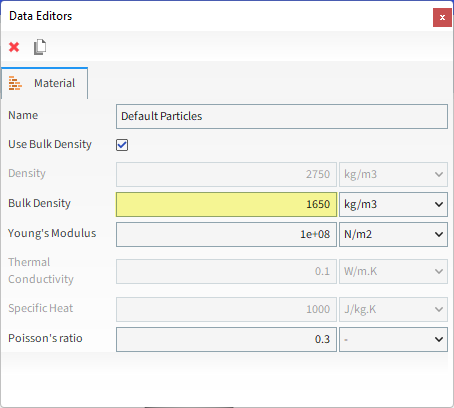
From the Data panel, under Materials select Default Particles and then from the Data Editors panel, change the following: Bulk Density.
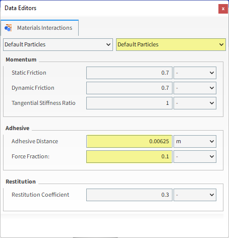
Now let's set the interaction properties for the materials:
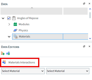
Select Materials Interactions from the Data panel. The Data Editors panel then displays the editable parameters.
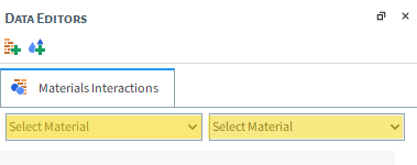
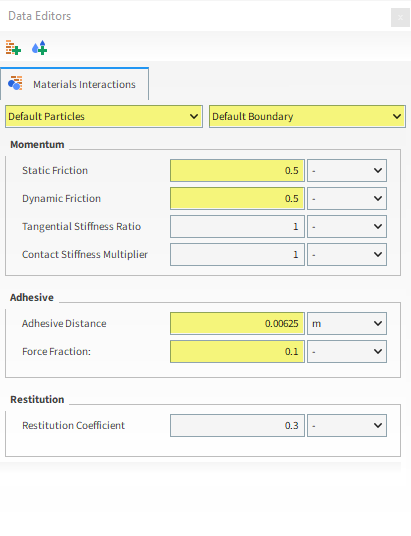
From the left drop-down list, select Default Particles, and from the right drop-down list, select one of these pairs: Default Boundary or Default Particles.
Adjust the parameters for each pair combination according to the values shown as follows:
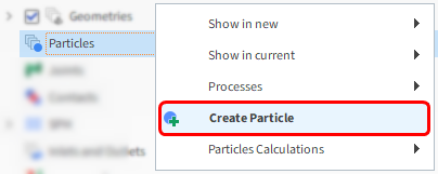
For the Particles step, we will create a new sphere-shaped particle group with some added rolling resistance.
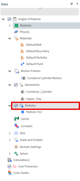
From the Data panel, right-click Particles and then select Create Particle. A new particle group is created under Particles.
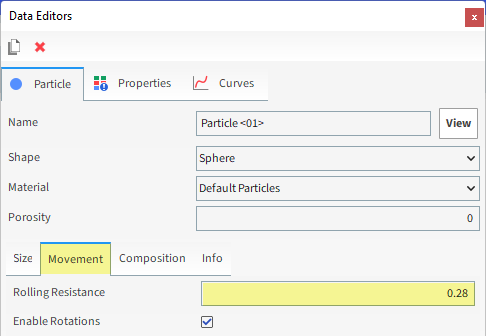
Select the newly created Particle <01> entry, and then from the Data Editors panel, modify the parameters as specified on the following steps.
From the Size sub-tab, define Size (in m).

From the Movement sub-tab, define Rolling Resistance.
To visualize the new particle, click View. A new Particle Details window will appear showing you the (transparent) particle geometry, its geometric center (yellow dot), and its center of mass (blue dot).
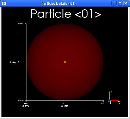
Note: The geometric center and center of mass coincide when the density is uniform throughout the particle (as shown).
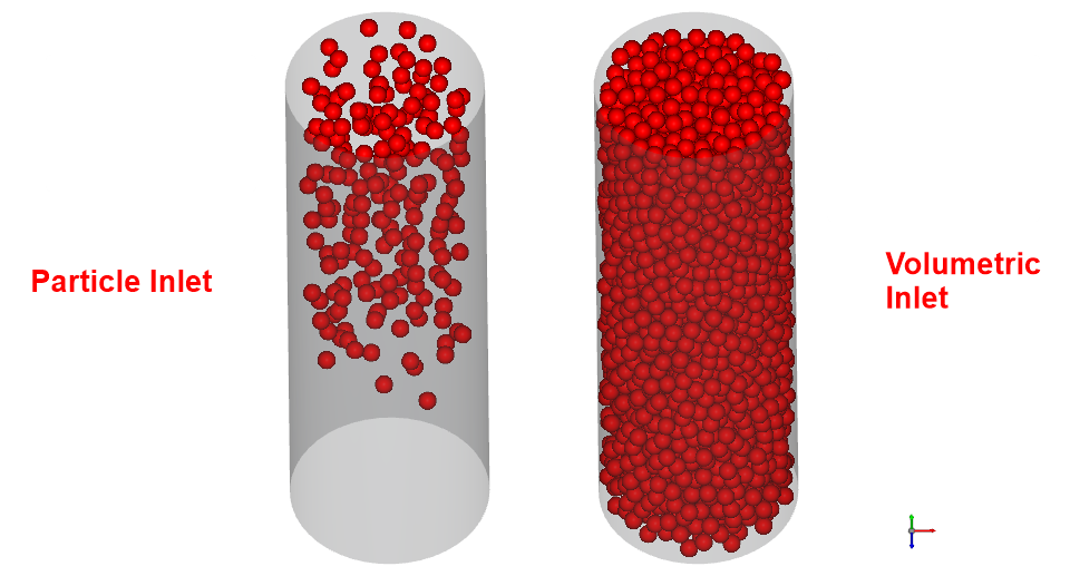
For the Inlets and Outlets step, we will create a Volumetric Inlet input, which enables us to inject a sphere-like ball of closely packed particles into the simulation all at one time.

When compared with the original Particle Inlet method (used in Tutorial 01), using Volumetric Inlet has the primary benefit of ensuring that the particle bed will already be formed in the cylinder at the start of the simulation.
When defining a Volumetric Inlet input, it is important to understand the following components:
Seed Coordinate: Location of a point around which layers of particles are built.
Gap Scale Factor: How closely the particles are to each other when they build around the Seed Coordinate.
Mass: The target mass of particles that you want to be built around the Seed Coordinate.
Bounds : Defines the physical limits by which the particle layers will be constrained. Specifically:
The limits must include Box Bounds, which can be defined manually using coordinates, or can be automatically calculated by Rocky using the limits of one or more Geometries that you select.
The limits may also include the walls of one or more Geometries within your simulation.
Time: The Time sub-tab contains optional time settings for Volumetric Inlets that can improve your simulation project:
Injection Time: Set the simulation time at which the particle injection occurs.
Periodic: When enabled, Periodic allows for a periodic injection of particles into the simulation. Period Time defines the period duration and Stop Time defines the simulation time when periodic injection stops.
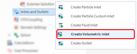
For this tutorial, we'll create a Volumetric Inlet constrained only by the Cylinder Wall.
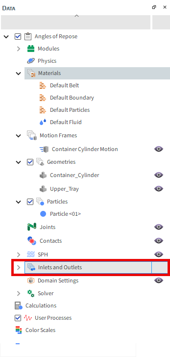
From the Data panel, right-click Inlets and Outlets and then select Create Volumetric Inlet. A new Volumetric Inlet <01> entry is created under Inlets and Outlets.
Select the newly created Volumetric Inlet <01> entry, and then from the Data Editors panel, modify the parameters as specified below:
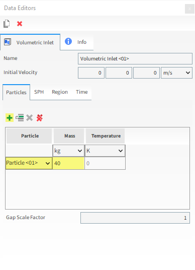
From the Particles sub-tab, click the Add button (green plus) to create an entry row.
Select the Particle <01> group name from the drop down list and then define the Mass in kilograms (as shown).
Leave the Gap Scale Factor as 1 (default) so that the particles are injected as closely together as possible.
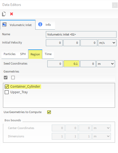
From the Region sub-tab, define the Seed Coordinates.
From the Geometries box, enable the Container_Cylinder checkbox.
Enable the Use Geometries to Compute checkbox.
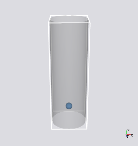
You can visualize the Seed Point you configured in the previous step in a 3D View window.
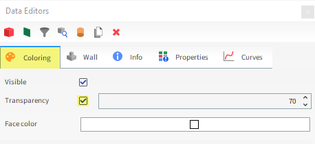
Since the Seed Coordinates were set to be inside the cylinder, we first have to enable its Transparency to be able to see the Seed Point.
From the Workspace, select a 3D View window (or create a new one).
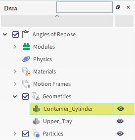
From the Data panel, select the Container_Cylinder geometry.
From the Data Editors panel, select the Coloring tab and then enable the Transparency checkbox.
From the Data panel, reselect the Volumetric Inlet <01>.
You can now visualize the Seed Point (blue dot) and geometry bounds (white box) in the 3D View window.
Now let's set the Solver parameters:
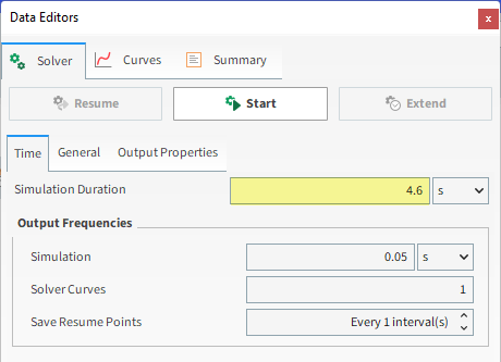
From the Data panel, click Solver and then from the Data Editors panel, ensure that the Solver tab is selected.
From the Time sub-tab, define the Simulation Duration.
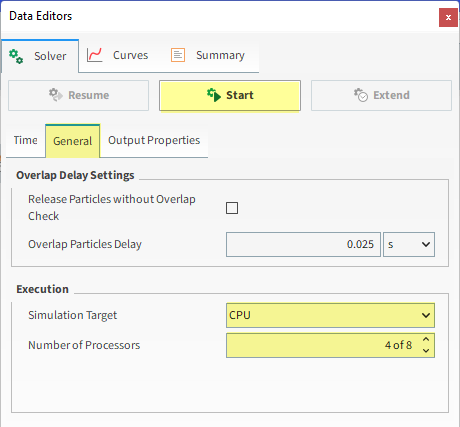
From the General sub-tab, select CPU (or GPU/Multi GPU) as Simulation Target, and then set the Number of Processors (or Target GPU(s)). For this tutorial, CPU will be faster due to the low particle count.
Click the Start button to begin processing.
Once you click Start, the Simulation Summary window will be displayed.
This window will disappear on its own, then processing begins.
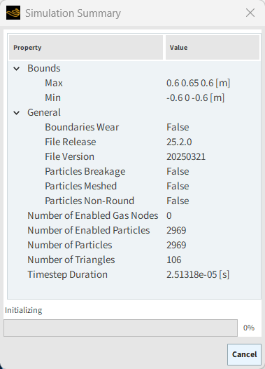
Tip: You can also review this information from the Solver | Summary tab.
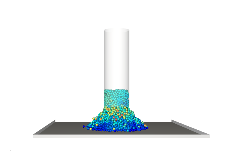
To visualize the simulation as it's processing:
From the Window menu, click New 3D View.
Click the Refresh button (or use the Auto Refresh checkbox).
The speed of the simulation depends upon various factors such as:
The particle shape and the number of vertices used to define the shape
Number of contacts in the simulation domain at any time
Number of mesh elements used to define the geometry
Smallest particle size and material stiffness
Frequency of file output
This completes Part A of this tutorial.
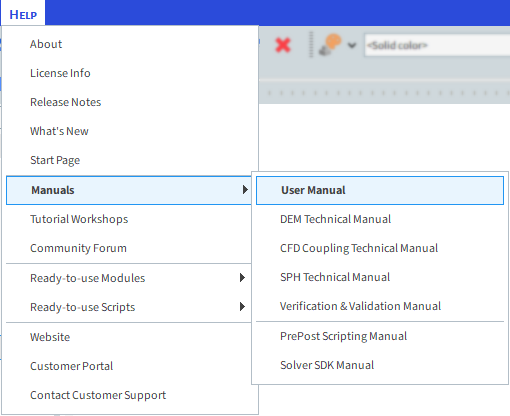
For further information on any topic presented, we suggest searching the User Manual, which provides in-depth descriptions of the tools and parameters.
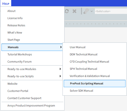
To access this manual, from the main Toolbar click Help, point to Manuals, and then click User Manual.
Rocky was used to set up and process a simulation of a static angle of repose (SAOR) test.
Note: Even though this tutorial involves running only one SAOR test, other simulations must be done in order to calibrate the particle model in full.
During this tutorial, it was possible to:
Set up a constant adhesion model
Change materials and interactions values
Define a Volumetric Inlet Input
Process the simulation
What's Next?
Now that you have set up and processed this simulation, you are ready to move on to Part B and post-process this project.
The purpose of this tutorial is to calculate the Static Angle of Repose (SAOR) using two methods: manually using Cross Plots and automatically using a Python script.
We will continue from where we left off in Part A.
You will learn how to:
Use a cross plot to measure the SAOR
Open the PrePost Script panel
Import and run a saved Python script
Interpret the results from the executed script
Modify the Python script
And you will use these features:
Cross Plot window
PrePost Script panel
PrePost Scripting Manual
Important: Even though this tutorial involves running only one SAOR test, other simulations must be done in order to calibrate the particle model in full.
If you completed Part A of this tutorial, ensure that the Rocky project is open. (Part B will continue from where Part A left off.)
If you did not complete Part A, do all of the following:
Download the
dem_tut02_files.zipfile here .Unzip
dem_tut02_files.zipto your working directory.Open Rocky 2025 R2. (Look for Rocky 2025 R2 in the Program Menu or use the desktop shortcut.)
Important: To make use of the Rocky project file provided, you must have Rocky 2025 R2 or later. If you have an earlier version of Rocky, please upgrade Rocky to the latest version or complete Part A from scratch.
From the Rocky program, click the Open Project button, find the dem_tut02_files folder, then from the tutorial_02_pre-processing folder, open the tutorial_02_pre-processing.rocky file.
Process the simulation. (From the Simulation toolbar, click the Start button.)
Now that the project has completed processing, we can begin to analyze it. Let's start with the manual method first.
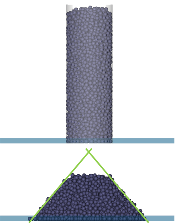
In this method, the Static Repose Angles (green lines) will be calculated manually by following these steps:
Generation of a plot with the particle distribution along X and Y directions
Measurement of the length and height using the chart scale
Calculation of the angles using trigonometric relationships
The Cross Plot is used to create a scatter plot, which allows you to compare two properties of the Particles/Geometry one on the X-axis and another on the Y-axis for a given Output.
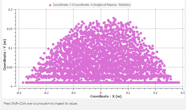
In this tutorial, we will use a Cross Plot to see the projection of the particles pile in the XY plane. In order to do that, the Particle Y-Coordinate will be plotted against the Particle X-Coordinate.
To create the Cross Plot, do all of the following:
From the Window menu, click New Cross Plot, or use the shortcut Ctrl+R.
From the Data panel, select Particles and then from the Data Editors panel, select the Properties tab.
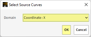
Click and drag Coordinate: Y over the plot window and then release.
From the Select Source Curves window that appears, select Coordinate: X from the Domain drop-down list, and then click OK.
Unlike the (Multi) Time Plot, which shows a single value per output for all the Particles, the Cross Plot shows all the Particles' values, but for only a single Output.
You can choose what instant to analyze using the Time toolbar.
Select the Time at 4.6 s to measure the Static Repose Angles.
The result is shown below.
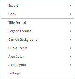
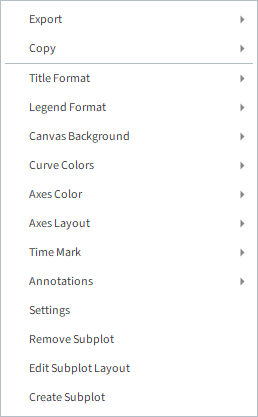
Rocky plots can be edited by right-clicking anywhere on the plot grid.
Cross Plot
Multi Time Plot
Export and Copy: Copy the plot or data; save the plot as a .png, .bmp or .jpg image file; or save a .csv data file.
Title Format: Display/hide the plot title, and edit it.
Legend Format: Display/hide the curves legend, and edit it.
Canvas Background: Change the plot area color and display/hide grid lines.
Curve Colors: Select curves coloring method: one color for each curve (Unique), identical colors for the same curves in the same or different entities (Particles/Geometries/Processes) (Property Based), or identical colors for the same or different curves in the same entities (Entity Based).
Axes Colors: Enable/disable the axis coloring according to the curve color.
Axes Layout: Toggle between independent axes for each curve (By Property), or a single axis for the same units (By Quantity).
Time Mark: Enable/disable the vertical dotted line synchronized with the selected instant in the Time toolbar.
Annotations: Add a custom text over the plot at any XY point.
Settings: Open the Windows Editor panel for additional controls.
Now, let's modify and re-scale the plot:
Right-click the cross plot view and then select Settings. (Or in the top left corner of the plot, select the Configure Window icon.)
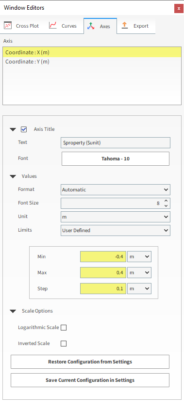
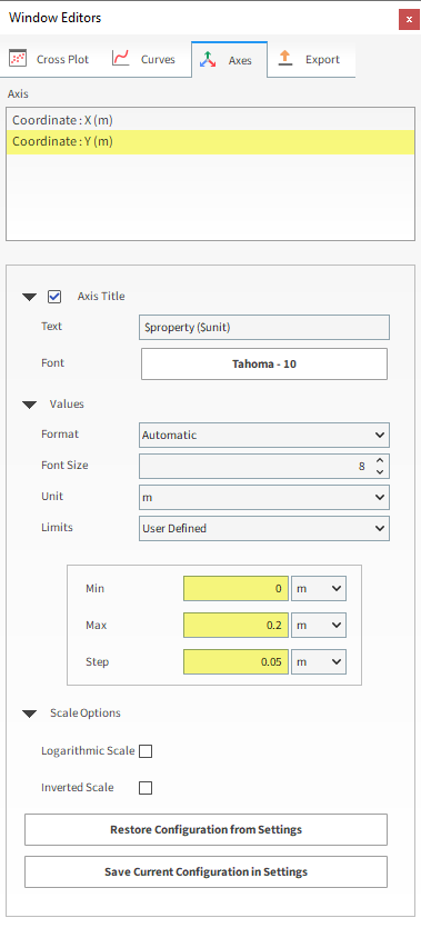
In the Window Editors panel, select the Axes tab, and then under Axis, multi-select both properties.
Under Values, change the Limits option to User Defined.
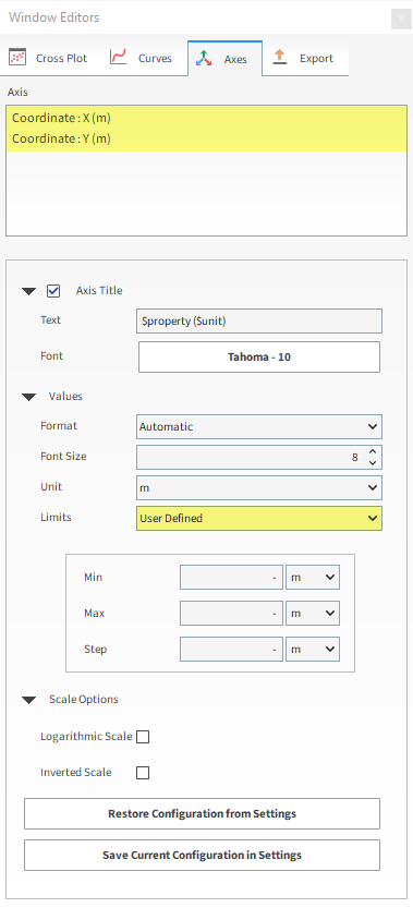
Set the value for Min, Max and Step for the two separate axes as shown below.
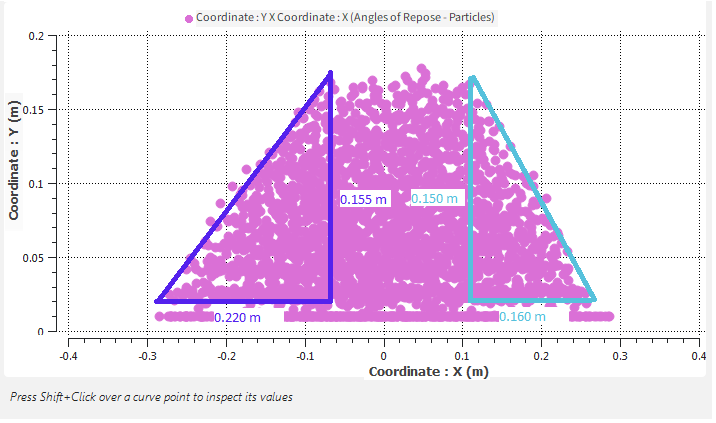
SAOR (1): Δx= 0.220 m; Δy= 0.155 m
SAOR (2): Δx= 0.160 m; Δy= 0.150 m
Note: The values you end up with in your project may vary slightly from the ones shown in this tutorial.
Once the values are measured, simple calculations can be done outside of Rocky using a spreadsheet or calculator:
SAOR(1): Δx= 0.220 m; Δy= 0.155 m
SAOR=atan(0.155/0.220) ~ 35.2°
SAOR (2): Δx= 0.160 m; Δy= 0.150 m
SAOR=atan(0.150/0.160) ~ 43.1°
Although these values were measured using the cross plot's axis scale, they can be measured using the mouse. To do that, hold the Shift key and then click the plot to show the cursor's value.
You can also post-process your results automatically by using a Python script.
Important: The provided script was designed for cases with higher particle counts than what was simplified for this tutorial. As a result, tutorial results may vary significantly.
In this method, the Static Angle of Repose (SAOR) will be calculated using the following steps:
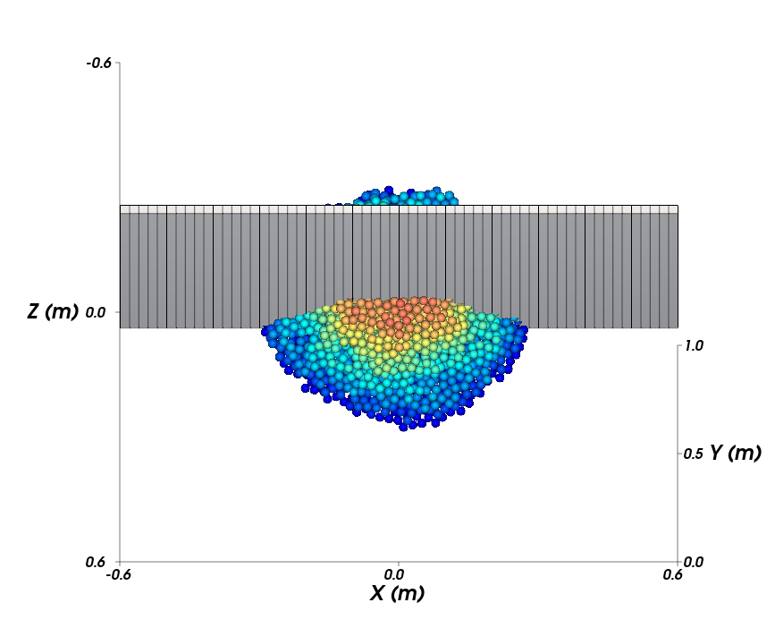
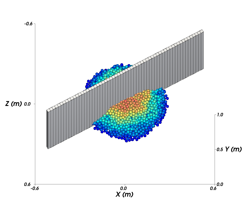
At a given output, a parallelepiped slice is divided into N vertical cells and placed at the pile center (as shown).
In each of these cells, the maximum particle height is collected.
Then, the parallelepiped slice is rotated 10 degrees around the vertical axis (Y-direction), and the maximum height of each cell is collected again. This step is repeated 36 times.
Using the average of the collected maximum heights for each cell, a regression line is created and the Static Angle of Repose is calculated.
In Rocky, you can automate frequent tasks in one of two ways:
Within Rocky, you can record Scripts of the exact steps you take in the user interface.
Outside of Rocky, you can write Scripts using the Python programming language that makes use of the PrePost Scripting.
Although they are generated in different ways, both methods can be played (executed) in the PrePost Script panel.
For this tutorial, we will focus on using a previously created script.
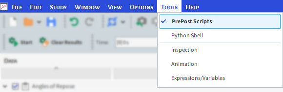
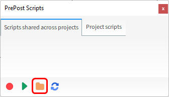
To start, show the PrePost Script panel by selecting it from the Tools menu.
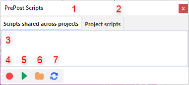
(1) Scripts shared across projects: Lists the scripts that can be used for any Rocky project.
(2) Project scripts: Lists the scripts that can be used for this project only.
(3) Lists all available scripts that are saved in the default folder for the selected tab.
(4) Record Script: Creates a script by recording the commands you execute manually in the user interface.
(5) Playback PrePost Script: Executes the selected script.
(6) Open PrePost Scripts Directory: Based upon the selected tab, opens the default folder where scripts are saved.
(7) Reload PrePost Scripts from the Filesystem: Refreshes the available scripts list based upon the default folder for the selected tab.
(8) Help: Displays some PrePost Script assistance content.
Tip: More PrePost Script panel content is available in the User Manual. (From the Help menu, point to Manuals, and then click User Manual.)
The Scripts shared across projects tab of the PrePost Script panel will show all the scripts you have saved in Rocky's default folder: %HOMEPATH%Documents\Rocky\Scripts.
Now, let's add the provided script to this panel and run it:
Ensure the Scripts shared across projects tab is selected.
Click the Open Scripts Directory button. This should take you to the Scripts folder listed above.
From dem_tut02_files folder you downloaded earlier, find the script folder and then copy and paste the provided script script_calibration_SAOR.py to the folder you just opened.
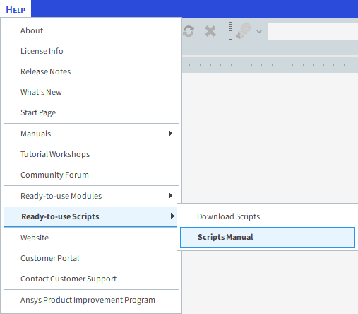
Note: The Static Angle of Repose script available in this Rocky Tutorial is only an example. To see all necessary information about the Calibration Suite and the SAOR script: from the Ansys Rocky Software, click Help, point to Ready-to-use Scripts and click Scripts Manual.
The new script will appear in the PrePost Scripts panel on the Scripts shared across projects tab (as shown).
With this new script selected, click the Playback Script button (as shown).
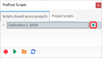
After the script finishes the calculation, the resulting plot will be displayed:
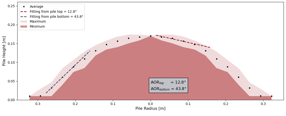
The dashed regression lines are used to compute the SAOR of the pile.
The black dots represent the average of the maximum heights for each vertical cell.
The dark red area represents the minimum of the maximum heights for each vertical cell.
The light red area represents the maximum of the maximum heights for each vertical cell.
Note: This script was designed for cases with higher particle counts than what was simplified for this tutorial. As a result, your tutorial results may vary significantly.
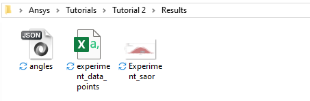
In addition, a Results folder is created in the same place as the Rocky project.
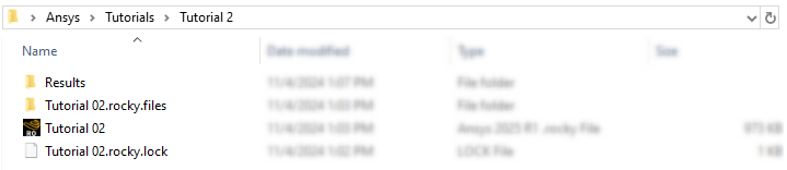
This folder contains the following files:
Experiment_saor.png: The output image of the script.
experiment_data_points.csv: File containing the points used for fitting the lines.
angles.json: Text file containing the calculated angles.
The provided script is based on Calibration 1: Static Angle of Repose test of the Rocky Calibration Suite.
Further information about this calibration test or other available calibration tests can be found in the Rocky Calibration Suite page.
As previously shown, the SAOR is calculated from the result of two linear regressions, one starting from the bottom of the pile and another one starting from the top of the pile.
Both linear regressions are performed initially with minimum number of points. Then, more points are iteratively added to the regressions until certain conditions are fulfilled. Such details are explained in the Calibration 1: Static Angle of Repose documentation.
The more particles you have, the better your results will be and the closer will be the SAOR calculated From Top to the one calculated From Bottom.
Tip: A smaller Particle Size or a larger Cylinder will increase particle count.
For additional particle calibration tests, consider making use of the following resources, both of which are available on the Customer Portal.
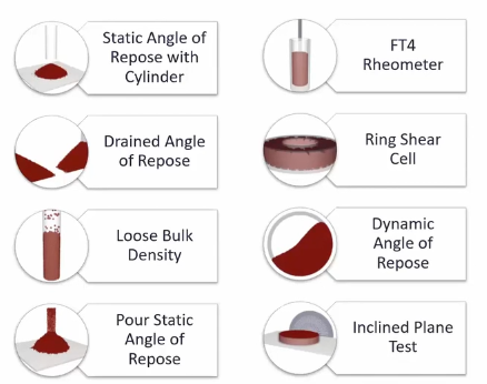
The Rocky Calibration Suite contains:
Eight pre-made Rocky projects representing common bench tests
Simplified project setup using pre-processing scripts
Automatic post-processing reports
The Material Wizard can be used as a time-saving starting point for your calibration process. For more details access the Material Wizard Page.
You can change some parameters within the script to have a better resolution of your repose angles calculations.
Note: The Static Angle of Repose script available for download and the workflow presented to modify the script in this Rocky Tutorial are only examples. All information about the Rocky Calibration Suite and its decks, including the SAOR script, are available in the Scripts Manual. From the Ansys Rocky Software, click Help, point to Ready-to-use Scripts and click Scripts Manual.
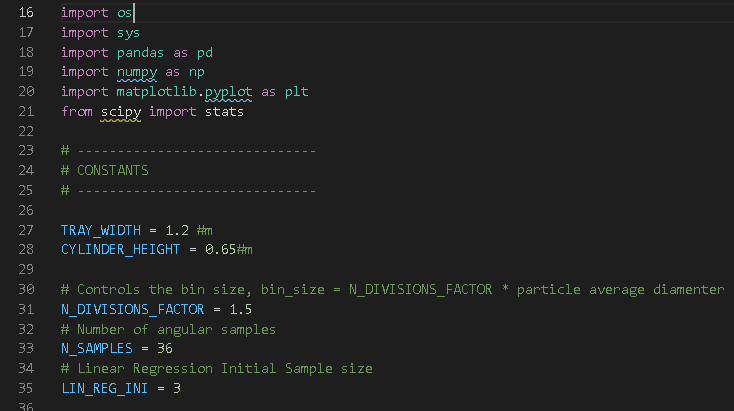
The main parameters are:
N_DIVISIONS_FACTOR (line 31):
Controls the cell size, which is defined by N_DIVISIONS_FACTOR Particle Size. As a consequence, the higher the factor, the bigger the cell size.
The default value is 1.5.
N_SAMPLES (line 33):
For each SAOR calculation, this defines the number of times the parallelepiped rotates and collects the maximum height.
The default value is 36, which rotates the parallelepiped 10 degrees for each collection.
Increasing this number (thereby reducing the angle of rotation) will give you more points to average.
LIN_REG_INI (line 35):
Initial number of points for the linear regressions.
The default value is 3.
To modify the script, do the following:
From the PrePost Script panel, from the Scripts shared across projects tab, click the Open PrePost Scripts Directory button.
From the directory dialog, right-click the script file you want to edit, and then open it with your favorite Python editor. (For example, Visual Studio Code.)
Modify it as desired, and then save the file as a .py extension.
Important: In order for Rocky to recognize it, the script file name must begin with script_.
For further information about the Rocky Calibration Suite, we suggest searching the Rocky Scripts Manual.
To access it, from the Rocky Help menu, point to Ready-to-use Scripts, and then click Scripts Manual.
From the Rocky Scripts Manual you can find information about the Coating Visibility Wizard, Material Wizard, General Scripts, and the focus of this Tutorial, the Calibration Suite.
For further information about Rocky scripting, we suggest searching the Rocky PrePost Scripting Manual.
To access it, from the Rocky Help menu, point to Manuals, and then click PrePost Scripting Manual.
To see the list of classes and methods available for scripting, navigate through the Class Reference section.
Tip: Additional classes and methods for scripting are available in the Rocky code. To access these, from the Rocky Tools menu, enable the Python Shell panel.
This completes Part B of this tutorial.
For further information on any topic presented, we suggest searching the User Manual, which provides in-depth descriptions of the tools and parameters.
To access these options, from the main Toolbar click Help, point to Manuals, and then click User Manual.
Rocky was used to verify the repose profile of particles in order to calculate the Static Angle of Repose.
Note: Even though this tutorial involves running only one SAOR test, other simulations must be done in order to calibrate the particle model in full.
During this tutorial, it was possible to:
Use a Cross Plot to manually measure the angles
Use the PrePost Script panel to run a Python script that measured the angles automatically
Find and make use of the PrePost Scripting Manual for modifying Python scripts
What's Next?
Now that you understand the basics on how to set up a script, you are ready to move on to Part C and learn about PrePost Scripts and the Rocky Scheduler.
The purpose of this tutorial is to study how the Static Angle of Repose (SAOR) behaves using different Static and Dynamic Frictions for the particle-particle interactions.
Note: This tutorial can be continued from either Part A or Part B.
You will learn how to:
Save the project setup parameters without the simulation results
Use input variables to parameterize materials interactions properties
Schedule scripts to run automatically before and after the simulation
Use the Rocky Scheduler to run multiple Rocky projects in sequence
And you will use these features:
Input Variables
PrePost Scripts
Materials Interactions
Rocky Scheduler program
If you completed either Part A or Part B of this tutorial, ensure that one of those Rocky projects are open. (Part C can continue from where either of these parts left off.)
If you did not complete Part A nor Part B, ensure that you have downloaded and extracted the dem_tut02_files folder, and then open the tutorial_02_pre-processing.rocky project.
Important: To make use of the Rocky project file provided, you must have Rocky 2025 R2 or later. If you have an earlier version of Rocky, please upgrade Rocky to the latest version, or complete the setup portion of Part A from scratch.
Note: You do not need to process the simulation for this particular tutorial.
In this tutorial, we want to vary the Static and Dynamic Friction coefficients of the particle-particle interactions and see how that changes the particle behavior.
To do this without losing the prior simulation's results, we will create multiple, similar projects and change only the two friction values in the new ones.
To avoid recreating these new projects from scratch, we will create a copy of the current project's setup parameters, and specifically NOT copy its results.
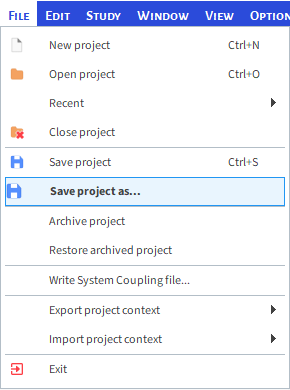
From the File menu, click Save project as....
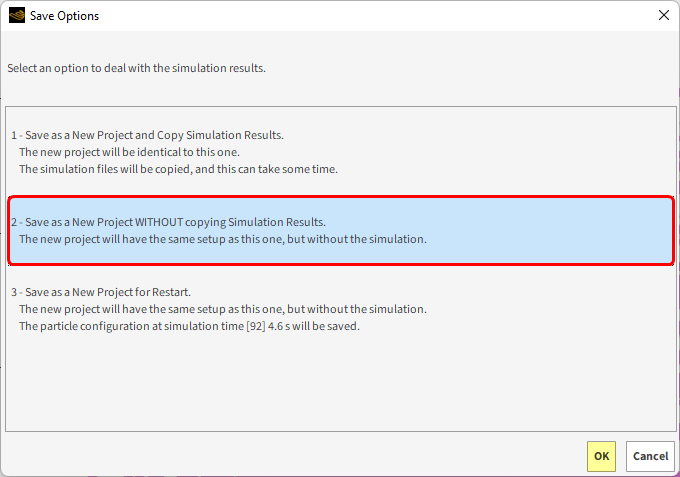
From the Save Options dialog, click Save as a New Project WITHOUT copying Simulation Results, and then click OK.
We want to save the project in another folder so the current Results folder won't be rewritten by the newly created project results.
We also want to name this new file in a specific way so that it is easier to track multiple copies later.
To accomplish these tasks, do the following:
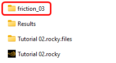
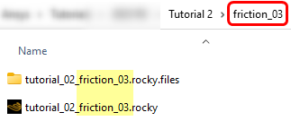
From the Save File window, create a new folder named friction_03 in the same location as the original project (as shown).
Double-click the new folder to open it.
Enter tutorial_02_friction_03.rocky for the File name, and then click Save.
For this tutorial, a single Input Variable will be set up for both Static Friction and Dynamic Friction.
For Input variables, you can enter into the parameter text fields a variable name on its own.
In this way, you can create dynamic relationships between parameters, and then change and update placeholder values quickly.
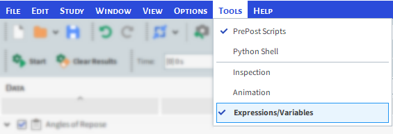
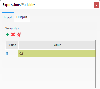
First, enable the Expressions/Variables panel by selecting it from the Tools menu.
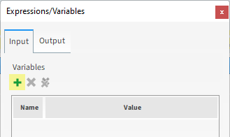
From the Expressions/Variables panel, ensure the Input tab is selected, and then click the Add button.
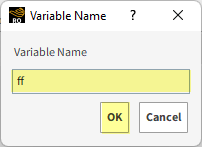
From the Variable Name dialog, set the Variable Name as ff (as shown), and then click OK.
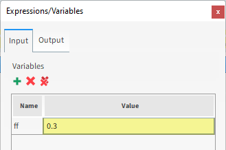
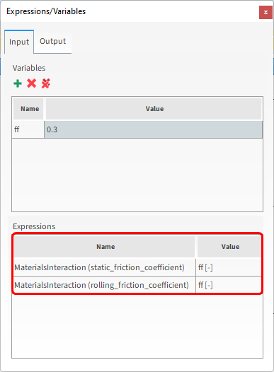
From the entry row that was added, double-click the Value, and then set it to 0.3 (as shown).
To assign the variable to the interaction properties, do the following:
From the Data panel, click Materials. From the Data Editors panel, select Materials Interactions tab. The editable parameters are displayed.
From the left drop-down list, select Default Particles, and from the right drop-down list, select Default Particles.
Type ff in the Static Friction text box.
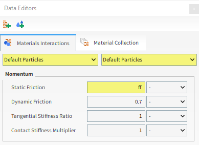
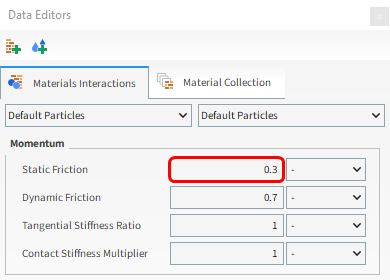
When you click away from this field, the Static Friction field will show the value you set for the ff variable (as shown).
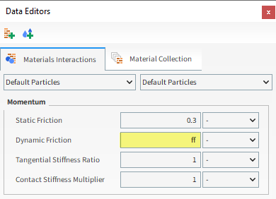
Repeat for the Dynamic Friction.
Whenever you use an Input Variable to define a parameter, the Expressions/Variables panel lists which variables were used for which parameters (as shown).
Next, we want the script we used in Part B to automatically run and save the output files right after the simulation is processed.
To do so, we must save it in the Project scripts tab, and then define it as a Post Script:
Scripts saved to the Project scripts tab are eligible for running automatically in two ways:
Right BEFORE the simulation starts processing (Pre Script)
Right AFTER the simulation is done processing (Post Script)
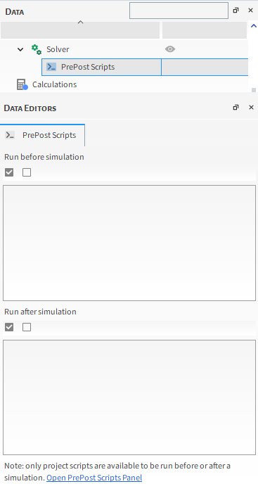
This is done through the PrePost Script sub-entity on the Data panel under the Solver entity (as shown).
In this way, you can further automate your setup and post-processing tasks, especially when running many similar kinds of cases.
Now, we will set this script to automatically run right after the simulation completes.
Ensure the PrePost Scripts panel is still shown. (From the Tools menu, select PrePost Scripts.)
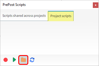
From the PrePost Scripts panel, select the Project scripts tab and then click the Open Scripts Directory button (as shown).
From the dem_tut02_files folder you downloaded earlier, find the script folder, and then copy and paste the provided script script_calibration_SAOR.py into the directory you just opened.
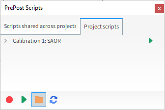
The new script will appear in the PrePost Script panel on the Project scripts tab (as shown).
Now, we will set this script to automatically run right after the simulation completes.
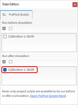
From the Data panel, expand the Solver entity and then select PrePost Scripts.
From the Data Editors panel, within the Run after simulation list, enable the Calibration 1: SAOR checkbox (as shown).
Save the project.
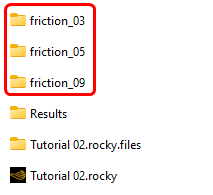
For this tutorial, we will run three cases in addition to the original case that we analyzed in Part B.
We already have the first copy defined (tutorial_02_friction_03.rocky), so let's now use it to create two more project copies.
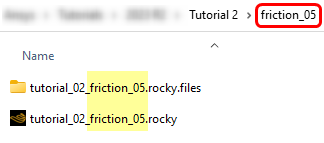
In the same root folder where you saved your original project, create another new folder named friction_05.
In Rocky, from the File menu, click Save project as....
From the Save File dialog, find and open the new folder you just created, enter the File name as tutorial_02_friction_05.rocky, and then click Save.
From within this new copy, change Input Variable ff to 0.5 (as shown).
From the File menu, click Save project.
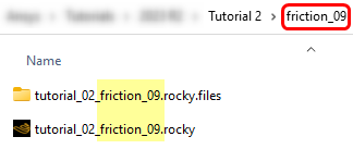
Repeat this process to create another folder called Friction_09 containing another project copy named tutorial_02_friction_09.rocky with both friction values (ff) changed to 0.9. (Remember to save your changes.)
You should now have the following three additional cases saved:
tutorial_02_friction_03.rocky: both frictions equal to 0.3
tutorial_02_friction_05.rocky: both frictions equal to 0.5
tutorial_02_friction_09.rocky: both frictions equal to 0.9
Once these cases are created, you can close Rocky.
We will now evaluate how the Angles of Repose behave in these cases.
For the original case we analyzed in Part B, we already have the Angles of Repose results.
If you did not complete Part B, you can review the results in the original_case_results folder, inside the dem_tut02_files you extracted previously.
We will get the results for these three new cases by running them through the Rocky Scheduler.
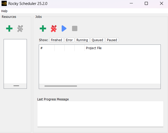
Open Rocky Scheduler 2025 R2.
Rocky Scheduler is a separate program that allows multiple simulation projects (Jobs) to be processed on specific hardware configurations (Resources) sequentially (one after the other) without having to use the Rocky User Interface (UI).
In this way, several cases can be run automatically without your constant involvement.
Each Job requires at least one Resource to be assigned to it.
Each Resource used will require one instance of the Rocky solver for processing.
Therefore, you are limited by your Rocky license as to how many Jobs you can process at once.
Most users have a single-instance Rocky license and can therefore process only one job at a time.
Only those users with unnumbered Rocky licenses can process many jobs at the same time.
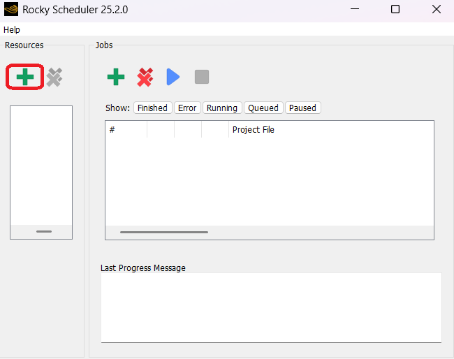
For this tutorial, we will add only one CPU resource and run the jobs sequentially.
To set up the Scheduler, from the Resources section, click the Add Resource (green plus) button.
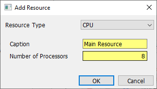
The Add Resource dialog appears with a Resource Type list that shows all the resources available on your computer (as shown).
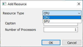
From the Add Resource dialog, set the Resource Type to CPU, enter the Caption and Number of Processors (as shown), and then click OK.
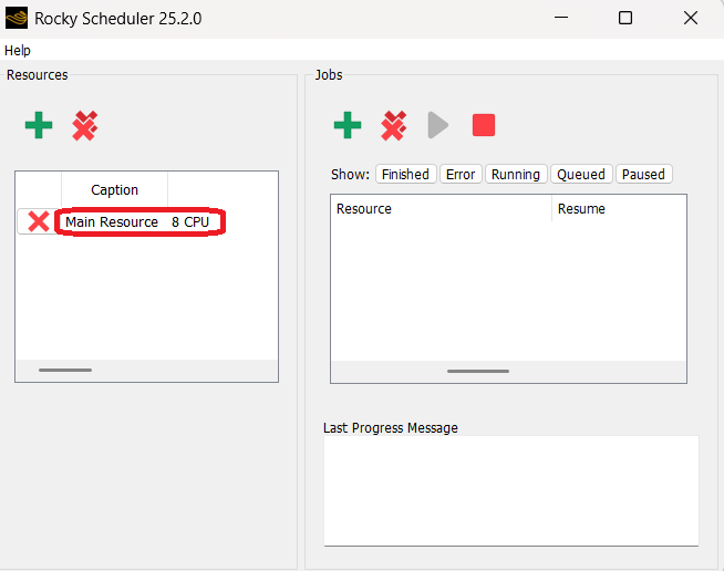
The resource you defined now appears on the Resources list.
Next, we will add our three projects to the Jobs queue:
From the Jobs section, click the Add Job (green plus) button (as shown).
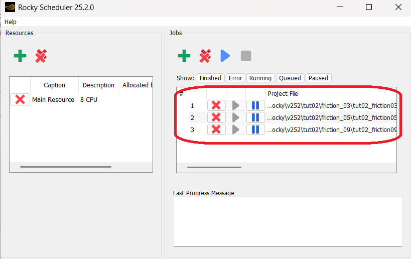
From the Choose Rocky project files dialog, select the tutorial_02_friction_03.rocky project we created previously, and then click Open.
Repeat this process for the tutorial_02_friction_05.rocky and tutorial_02_friction_09.rocky files. The three new jobs appear in the queue (as shown).
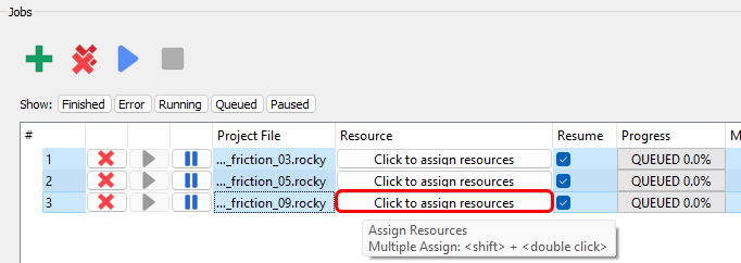
To assign the same Resource to all three jobs, do the following:
Multi-select all three jobs. (Hold the Shift or Ctrl key and then click each job to select it).
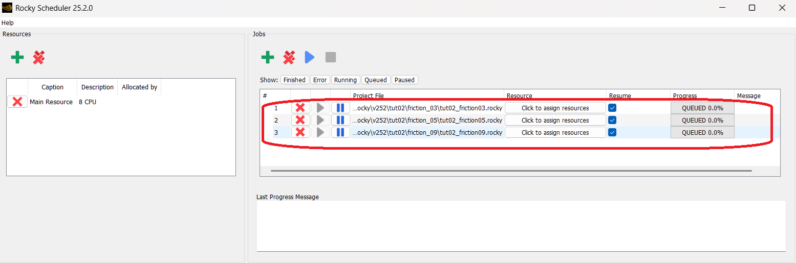
While holding the Shift key, double-click the last selected of the three Click to assign resources bars (as shown).
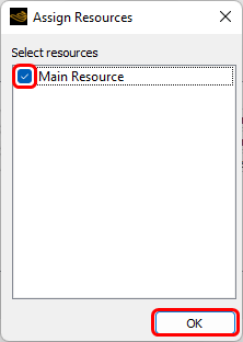
From the Assign Resources dialog, enable the Main Resource checkbox, and then click OK (as shown).
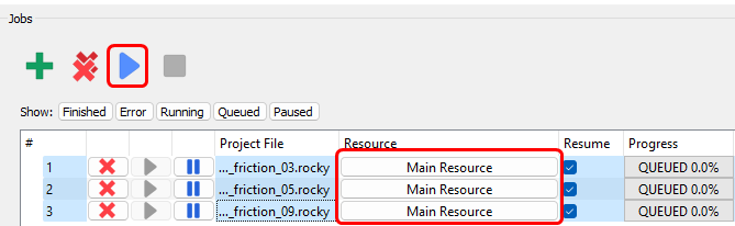
All three jobs should now list the same Resource (as shown).
Now, let's start the simulations:
Click the Start Scheduler button (as shown).
The first job in the list begins processing. You can view the Progress column to see the processing status and percentage complete.
RUNNING shows when the file is currently being processed (as shown).
QUEUED shows if the file is not currently processing but will once the resource is available.
PAUSED shows when the file has been partially run but isn't processing currently.
FINISHED shows when processing is complete.
ERROR shows when processing can't continue due to errors.
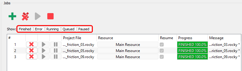
Tip: To filter the Jobs list by progress type, click the button you want from the Show list (as shown). To turn off a filter, click the same button again.
After all three jobs are done processing, all three Progress columns show FINISHED 100% and you will see that the Results folders were created inside of each of the created project folders.
Inside each folder there will be two files: angles.json and experiment_data_points.csv.
The angles.json files are shown below.
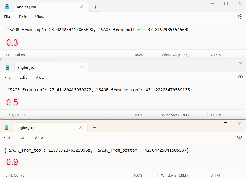
Note: When using the Scheduler, the figures are not generated. If you want to generate the figures, you must open each project in Rocky and run the script again.
From the values provided in the four .json files, a graph can be built outside of Rocky (as shown).
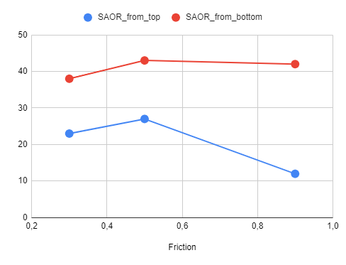
Note:
For sake of simplicity, the particle count of this tutorial was reduced.
Thus, the angle values you end up with in your real-world projects may vary significantly from the ones shown in this tutorial.
This is because the angles of repose calculations are very sensitive to the system resolution (proportion between the particle size and the cylinder size).
In order to achieve more accurate results you should increase particle count (reduce the particle size or increase the cylinder size).
This completes Part C of this tutorial.
For further information on any topic presented, we suggest searching the User Manual, which provides in-depth descriptions of the tools and parameters.
To access this manual, from the main Toolbar click Help, point to Manuals, and then click the User Manual.
The Rocky Scheduler was used to run multiple projects and analyze how the SAOR values vary when different particle-particle Dynamic and Static Frictions are used.
Note: Other simulations must be completed in order to calibrate the particle model in full.
During this tutorial, it was possible to:
Save the project without results to create a copy of just the setup parameters.
Use Input Variables to parameterize materials interactions properties.
Add a Project Script and then use PrePost Scripts to run it automatically after processing completes.
Use the Rocky Scheduler to run multiple projects sequentially.
What's Next?
If you completed this tutorial successfully, then you are ready to move onto the next tutorial.