


The main purpose of this tutorial is to use Workbench to set up a 1-Way coupled DEM-FEA simulation between Rocky and Ansys Transient Structural - Mechanical.
This Part A will cover Workbench project creation, Rocky project setup, and running the DEM simulation in Rocky.
Part B will cover 1-Way coupling with Transient Structural - Mechanical to calculate the FEA portion of the project.
The scenario considered in this tutorial is evaluating the structural integrity of a transfer chute given varying feeder belt speeds.
You will learn how to:
Create a Workbench project
Connect the Workbench project to both Rocky and Ansys Transient Structural - Mechanical
Set up the DEM portion of the project in Rocky to share data for later FEM analysis
Process and post-process the DEM results
And you will use these programs:
Ansys Workbench
Rocky
To complete this tutorial, you are required to have on a Windows machine, both of the following:
(1) A valid license for Ansys Mechanical 2025 R2, compatible with Transient Structural.
(2) Rocky 2025 R2 or later.
Important: This ADVANCED tutorial assumes that you are already familiar with the following programs and resources:
The Ansys Workbench platform.
If that is not the case, please refer to the Ansys Workbench user documentation for basic introduction about Workbench usage before beginning this tutorial.
The Rocky 2025 R2 program.
If this is not the case, it is recommended that you complete at least Tutorials 01 - 05 before beginning this tutorial.
Note: Ansys Rocky and Ansys Workbench integration is currently supported only on Windows and is automatically established during the installation process via Ansys Automated Installer.
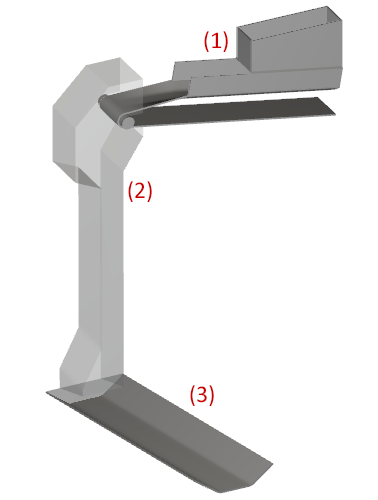
The geometries in this tutorial include the following components:
(1) Feed Conveyor
(2) Chute
(3) Receiving Conveyor
Note: The chute geometry will be imported into Workbench as a Discovery file. The conveyors will be added within the Rocky program.
To begin setting up the project, do the following:
Download the
dem_tut15_files.zipfile here .Unzip
dem_tut15_files.zipto your working directory.Open Ansys Workbench 2025 R2 (or later version).
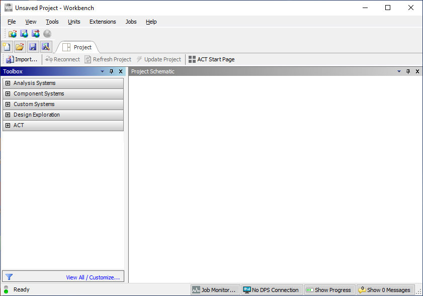
Save the empty Workbench Project from the File, Save As... menu item.
Tip: If you run into settings or procedures in these tables that you are not yet familiar with, please refer to the Rocky User Manual and/or other Tutorials (via the Introductory Tutorials and Advanced Tutorials) to find the detailed instructions you need.
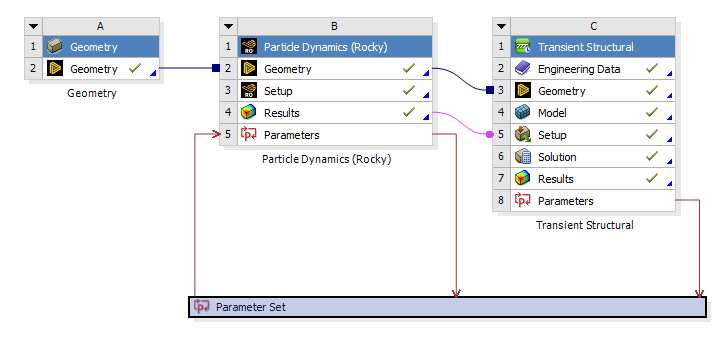
Use the information in the table below to start setting up your Workbench project:
Step Toolbox Entity Project Schematic Item Action A Component Systems ﹂Geometry
Drag and drop onto Project Schematic B Geometry ﹂Geometry
Import Chute.dsco from workshop_15_input_files C Analysis Systems ﹂Particle Dynamics (Rocky)
Drag and drop onto Geometry | Geometry D Analysis Systems ﹂Transient Structural
Drag and drop onto Rocky | Results E Rocky ﹂Results
Delete the link to Transient Structural | Model F Save the Workbench Project G Rocky ﹂Setup
Edit...
While performing the steps in the table above, note the following:
Dropping the Rocky block onto the Geometry component will automatically generate a connection between the Geometry and Rocky.
While Rocky is processing, you should not modify/save/close the connected Workbench session.
When Rocky interface opens (Step G), the linked geometry component is automatically imported from Ansys Discovery. In addition, the Boundary Collision Statistics module is automatically enabled with Forces for FEM Analysis option pre-selected.
Note: It also happens for the SPH Boundary Interaction Statistics and the Nodal Forces option. For this setup, it will not be used.
Now that the Workbench project is set up, let's define the Rocky project settings.
Since a coupled simulation with Ansys Mechanical will be carried out for this geometry part, it is important to refine the mesh so that the pressure field transferred to Mechanical has an adequate resolution for the desired structural analysis.
Every triangle node will provide x, y, z pressure components, which will then be applied as a load inside Mechanical.
To visualize and refine the mesh, do the following:
Drag and drop Geometries to the Workspace.
Use the information in the tables that follow to modify the Chute meshing and set up the Feed Conveyor.
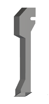
Step Data Entity Editors Location Parameter or Action Settings A Geometries ﹂Chute
Coloring Edges (Enabled) Wall | Transform Triangle Size 0.1 [m]


| Step | Data Entity | Editors Location | Parameter or Action | Settings |
|---|---|---|---|---|
| B | Geometries | Create Feed Conveyor template | ||
| C | Geometries ﹂Feed Conveyor | Feed Conveyor | Geometry | Transition Length | 1 [m] |
| Loading Length | 2.5 [m] | |||
| Belt Width | 0.6 [m] | |||
| … | Orientation | Alignment Angle | -90 [m] | ||
| Belt Incline Angle | 10 [m] | |||
| … | Skirtboard | Width | 0.5 [m] | ||
| Length | 1 [m] | |||
| Skirtboard Height | 0.3 [m] | |||
| … | Feeder Box | Drop Box Width | 0.5 [m] | ||
| … | Head Pulley | Face Width | 0.8 [m] | ||
| Diameter | 0.2 [m] | |||
| Offset to Idlers | -0.1 [m] | |||
On the Belt Motion sub-tab, define the Belt Speed.
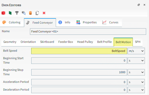
This will automatically create a new variable for this parameter, as indicated by the Variable Creation dialog.
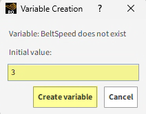
For the Initial value, input 3 m/s (as shown), and then click Create variable.
Creating this input variable will expose it as a parameter in Workbench, which we will make use of in Part B.
Verify the new input variable as follows:
From the Tools menu, ensure that the Expressions/Variables panel is enabled.

On the Expressions/Variables panel, the new BeltSpeed variable and value you defined is shown.
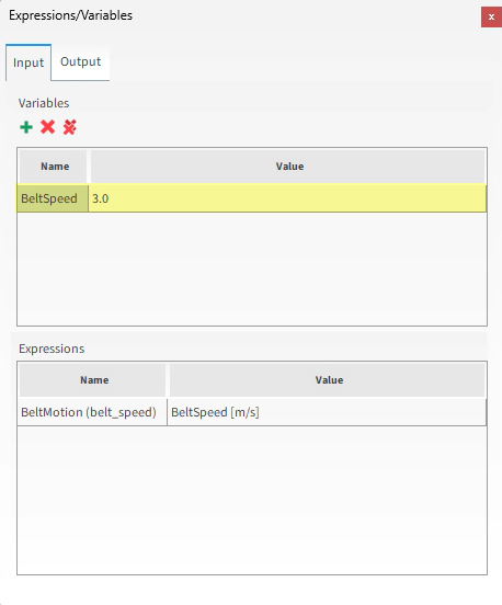
You may change the Value to see how this influences the Feed Conveyor geometry. However, for the purposes of this tutorial, please keep the value as 3.0 m/s.
Now that our feed conveyor is set up, we can create the receiving conveyor.
Use the table below to continue setting up your project.
Step Data Entity Editors Location Parameter or Action Settings A Geometries Create Receiving Conveyor template B Geometries ﹂Receiving Conveyor <01>
Receiving Conveyor | Geometry Length 5 [m] … | Orientation Belt Incline Angle 10 [deg] Vertical Offset -5 [m] Horizontal Offset -0.6 [m] Out-of-Plane Offset 0.2 [m]
For this tutorial, the default Materials and Materials Interactions settings will be used without changes.
Next we will add a rock-shaped polyhedron particle set in multiple sizes that will be injected through a Particle Inlet.
Use the information in the table below to continue setting up your project.
Step Data Entity Editors Location Parameter or Action Settings A Particles Create Particle B Particles ﹂Particle <01>
Particle Shape Polyhedron … | Shape Horizontal Aspect Ratio 1 Number of Corners 15 … | Size Add size row (x1) (1) Size | Cumulative % 0.15 [m] @ 100 [%] (2) ... 0.1 [m] @ 30 [%] C Inlets and Outlets Create Particle Inlet D Inputs ﹂Particle Inlet <01>
Particle Inlet Entry Point Feed Conveyor <01> … | Particles Add row (x1) (1) Particle | Mass Flow Rate Particle <01> ⯆ @ 300 [t/h]
For this Tutorial, transient loads on only the chute geometry will be exported to Ansys Transient Structural - Mechanical.
Follow the steps in the table below to set Wall Loads and Solver parameters.
Step Data Entity Editors Location Parameter or Action Settings A External Coupling ﹂Wall Loads
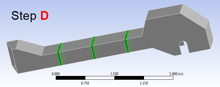
Wall Loads Select Walls | Chute (Enabled) Time Range Filter | Domain Range All ⯆ B Solver Solver | time Simulation Duration 10 [s] Output Settings | Time Interval 0.1 [s] … | General Execution | Simulation Target CPU ⯆
With a 3D View window opened, your Data panel and Workspace should look similar to the below image.

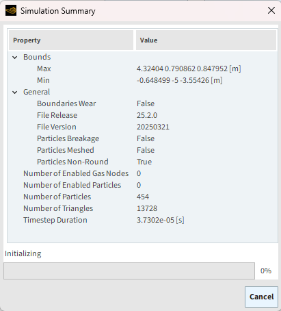
From the Solver entity, click Start.
The Simulation Summary screen appears (as shown), then processing begins.
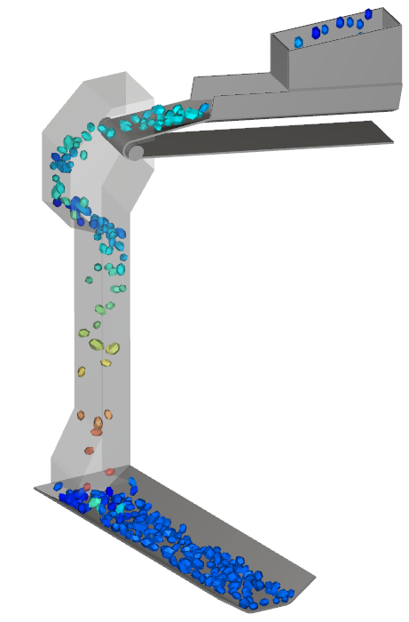
Tip: You can use the Auto Refresh checkbox to view in a 3D View window the results during processing.
Note: When the simulation processing is done inside Workbench as is done in this Tutoria all files are saved in the Workbench file directory, including the ones needed for Rocky.
One analysis you can do after the simulation is done processing is to quantify the force of the particles as they collide with the Transfer Chute. By plotting the Force : Z, we can visualize this quantity over time.
From the Data panel, under Geometries, select Chute.
From the Data Editors panel, select the Curves sub-tab, right-click Force : Z and then click Show curve in new Plot.
The result will be a new time plot showing the summed nodal forces observed by the Chute wall over the duration of the simulation.

Later in Part B of this tutorial, we will use the Force : Z of the chute geometry to help determine whether modifications made during parameterization are improving the design.
We will expose this parameter to Workbench by making it available on the Output tab of the Expressions/Variables panel.
Follow the steps in the table below to expose the Force : Z parameter for later analysis.
Step Item Location Parameter or Action Settings A Geometries ﹂Chute
Curves | Force: Z Drag and drop to Expression/Variables | Output B Expressions/Variables Output Force_Z Edit (button) C Edit Properties (dialog box) Operation on Curve average ⯆ Domain Range Time Range ⯆ Initial 3.5 [s] Final 10 [s]
Note that we have set the time range for the force output to start a few seconds into the simulation. This is to account for the time it takes for the particle flow to reach the chute.
Once processing is complete, do the following:
Save your Project.
Close Rocky.
Switch back to your Workbench project.
Note: Due to its connection with Workbench, nothing further is required in Rocky after processing is complete. There is no need to export any files. All necessary data transfers will happen in Workbench.
This completes Part A of this tutorial, in which through Ansys Workbench Rocky was used to set up and process a Transfer Chute simulation that will later be 1-Way coupled with Ansys Transient Structural - Mechanical.
During this tutorial, it was possible to:
Verify that Rocky is ready for coupling with Ansys.
Create a new Ansys Workbench project that connects an imported geometry to both Rocky and Ansys Transient Structural - Mechanical.
Set up and run the Rocky portion of the simulation through Workbench.
Ensure the collection of forces data for later FEM analysis.
Enable a DEM setup field to be later parameterized in Workbench.
Expose a DEM parameter to Workbench for later analysis.
Define what geometry load data to later share with Mechanical.
What's Next? If you completed this part successfully, then you are ready to move on to Part B and set up and run the FEA simulation based upon these DEM results.
The main purposes of this tutorial are to use Ansys Workbench to run a 1-Way coupled DEM-FEA simulation using Rocky and Ansys Transient Structural - Mechanical, and then analyze those results.
We will make use of the Rocky DEM results we created in Part A.
As a reminder, the scenario considered in this tutorial is evaluating the structural integrity of a transfer chute given varying feeder belt speeds.
You will learn how to:
Use Workbench to transfer DEM results from Rocky to Transient Structural - Mechanical
Set up and process the FEA simulation in Transient Structural - Mechanical
Analyze key input and output project parameters in Workbench
And you will use these programs:
Ansys Workbench, including the Parameter Set (Table of Design Points)
Ansys Transient Structural - Mechanical
To complete this tutorial, you are required to have in a Windows machine, both of the following:
(1) A valid license for Ansys Mechanical 2025 R2, compatible with Transient Structural.
(2) Rocky 2025 R2 or later.
Important: This ADVANCED tutorial also assumes that you are familiar with all of the following programs and resources:
The Ansys Workbench platform.
If that is not the case, please refer to the Ansys Workbench user documentation for basic introduction about Workbench usage before beginning this tutorial.
Note: Rocky and Ansys Workbench integration is currently supported only on Windows.
The Ansys Transient Structural - Mechanical program.
If this is not the case, please refer to the Ansys Mechanical user documentation for a basic introduction about Mechanical usage before beginning this tutorial.
If you completed Part A of this tutorial, ensure that the Ansys Workbench project you created is open. (Part B will continue from where Part A left off.)
If you did not complete Part A, do all of the following:
Download the
dem_tut15_files.zipfile here .Unzip
dem_tut15_files.zipto your working directory.Open Ansys Workbench.
Important: To make use of the Workbench project file provided, you must have Ansys 2025 R2 or any Rocky-supported version and Rocky 2025 R2 or later. If you have an earlier version of either of these programs, please upgrade to the latest version of Rocky and the latest version of Ansys that is supported by Rocky, or complete Parts A from scratch.
From the Workbench program, click the Open Project button, navigate to the tutorial_15_A_processing-rocky folder and open the tutorial_15_A_processing-rocky.wbpj file.
With the project open in Workbench, you are now ready to begin Part B.
Before we set up the Mechanical project, we need to update the results.
Follow the steps in the table below to transfer the DEM results into Workbench and open Mechanical with this data available.
Note: Step A is only necessary if you are using the already set-up tutorial_15_A_processing-rocky.wbpj project file that you downloaded together with the tutorial files.
Step Project Schematic Item Action A Rocky | Edit Necessary to ensure Workbench recognizes the Force : Z Output Parameter set in the Rocky Project. Close Rocky and return to Workbench. B Rocky | Setup Refresh C Rocky | Results Update D Transient Structural | Model Edit...
Use the information in the table below to set up your Mechanical project.
Step Outline Entity Details Location Parameter or Action Settings A Model ﹂Geometry
﹂Chute/Surface1
Definition Thickness 0.01 [m] B Model ﹂Mesh
Generate Mesh C Model ﹂Transient
Insert Fixed Support D Model ﹂Transient
﹂Fixed Support
Scope Geometry With the Face tool, multi-select the 12 faces (as shown on next slide) and then Apply E Model ﹂Transient
﹂Analysis Settings
Step Controls Step End Time 10 [s] Auto Time Stepping Off ⯆ Time Step 0.1 [s] F Model ﹂Transient
﹂Imported Load
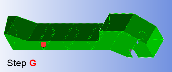
Insert Pressure G ... ﹂Imported Load
﹂Imported Pressure
Scope Geometry With the Mode of Box Select, select the whole chute (as shown) (35 faces) and then Apply Definition Define By Components ⯆ 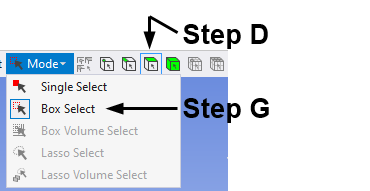
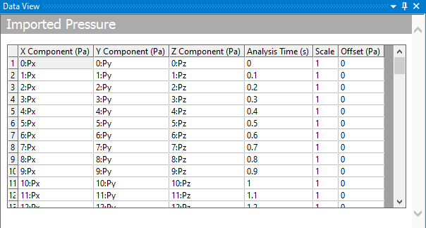
From the Data View panel, fill in the Imported Pressure table by defining the following components for each output recorded (X Component (Pa), Y Component (Pa), and Z Component (Pa)) as described below.
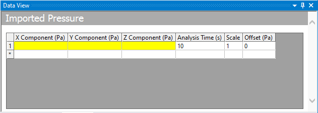
In the directory to which you have saved your Workbench files, navigate to the ../dp0/RockyEx/Rocky folder.
From within this folder, find the loadref.csv file and open it with a text editor (for example, Notepad).
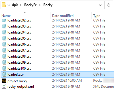
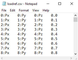
Select all of the content, and then copy it.
Return to Ansys Mechanical, and then on the first column and line of the Imported Pressure table, paste all of the information you copied. (Results shown below.)
Using this method enables you to skip defining the components for each exported file manually.
Note:For this method to work, your operational system language should be defined as English or another that consider "." as the separator for decimals. Otherwise, the Analysis Time column will automatically make a conversion and assume wrong values (for example, 0.1 will be assumed as 1).
The integration between Ansys Rocky and Ansys Workbench allows Forces to be automatically exported, but pressure still requires the manual export workflow described above.
Use the information in the table below to define which solutions to include in the calculations.
Step Outline Entity Details Location Parameter or Action Settings A Model ﹂Transient
﹂Solution
Insert | Deformation | Total Insert | Stress | Equivalent (von-Mises) B Model ﹂Transient
﹂Solution
Solve
The FEA simulation starts processing.
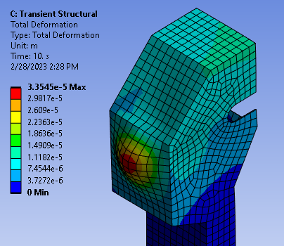
When the simulation concludes, the effects caused by the particles colliding with the chute surfaces can be easily seen:
Under Solution, select Total Deformation and then view the results (as shown).
Repeat for Equivalent Stress (as shown).
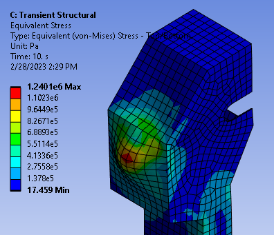
Tip: Use the Graph and the Tabular Data panel to see how the results vary through the simulation time.
It is possible to analyze variables in relation to others if we parameterize them.
Follow the steps in the table that follows to define the solutions we want to analyze as parameters.
Step Outline Entity Details Location Parameter or Action Settings A Model ﹂Transient
﹂Solution
﹂Total Deformation
Results Maximum Define as a parameter (P) by clicking the box B ... ﹂Solution
﹂Equivalent Stress
Save the project, close Mechanical, and return to Workbench.
The last part of this tutorial is to make use of Workbench's Design Points feature.
In Ansys Workbench, double-click the Parameter Set block.
From the Parameter Set tab, select the Outline Of All Parameters window.
Here, all the parameters created during the analysis are listed, no matter in which application they were created or if they are input or output parameters.
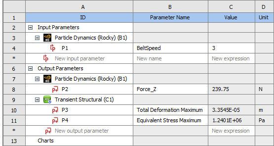
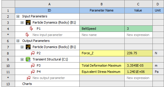
In the Outline of All Parameters window, both the input and output parameters we defined earlier in this tutorial are listed. Specifically:
Under Input Parameters, you can adjust the BeltSpeed of the Feed Conveyor we set up in Part A in Rocky (shown in green).
And see how it affects the results under Output Parameters (shown in yellow), including:
The resulting Force_Z output from Rocky due to the particles on the chute liner.
The Total Deformation Maximum and Equivalent Stress Maximum outputs we parameterized earlier in Mechanical.
These parameters can be directly changed to compare different scenarios, in order to provide you information on how to improve the chute design for the bulk material flow.
For example, you can also change and compare:
Particle-related quantities such as material density, tonnage, the particle geometry, the particle size distribution, and so on.
Chute structural quantities such as the number of supports, the material properties, supports, the overall design of the chute, and so on.
Now that we have analyzed the structural load on the original chute design, let's see how the results change when we change the input values.
Let's analyze what happens to the chute when we change the Feed Conveyor's BeltSpeed.
We will do this in the Table of Design Points by adding two new Design Points (DPs) and changing the input parameters.
Right-click DP 0 (the current Design Point) and then click Duplicate Design Point.
Repeat a second time to create another duplicate.
From the new DP 1 and DP 2 lines, define the P1 - BeltSpeed (as shown).
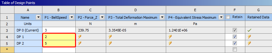
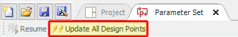
Run the new analyses by clicking the Update All Design Points button.
The new DPs will be run in both Rocky and Mechanical, and the resulting output parameters will be shown in this table for analysis.
Each DP is run sequentially as the previous is finished.
For each DP, Workbench will save the files (setup and results) if the Retain checkbox is enabled. If not, it will delete the results as soon as the simulation is done and the output parameters were obtained.
This is useful when you run several cases and are in danger of running out of space. You can then re-run only the best scenario cases (or the worst in case you want to identify failure scenarios).
Tip: For a more automated method of varying parameters to achieve defined design goals, you can also use Design Exploration. (Refer to Tutorial 12 for a step-by-step example.)
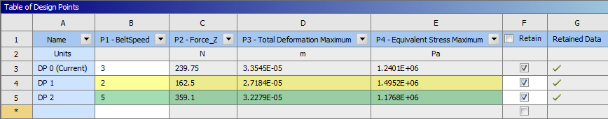
After the new DPs have been updated, we can look at the resulting output parameters and can see that the results match what we might have expected:
Reducing the feed conveyor belt speed (DP 1, in yellow) resulted in lower overall forces and stresses on the chute.
Increasing the feed conveyor belt speed (DP 2, in green) resulted in higher overall forces and stresses on the chute.
Tip: To open the applications for the new design points, you have to enable the Retain checkmark on the Table of Design Points.
This completes Part B of this tutorial, in which through Ansys Workbench / Ansys Transient Structural - Mechanical was used to set up and run a FEA simulation using the particle forces calculated previously by Rocky.
During this tutorial, it was possible to:
Make the Rocky DEM results available to Mechanical
Set up and process the FEA simulation in Mechanical
Analyze key input and output project parameters and set up new cases in Workbench
What's Next? If you completed this part successfully, then you are ready to move on to the next tutorial.