


This tutorial contains the following sections:
Molding is a process of forcing a preform or a parison (preshaped sleeve) into a mold cavity so that the preform assumes the shape of the cavity. There are numerous molding methods, including blow molding, compression and transfer molding, and slush and rotational molding. These methods differ in the formation of the preform and the filling of the mold cavity. Also, each processing method is suitable for a specific class of polymers.
Blow molding is an important processing method for molding hollow articles such as bottles. The preform is usually made by extrusion and forced between the mold halves by pressurization (blowing air). The polymer solidifies upon contact with the cold mold and the finished product is then ejected. The homogeneity and rheological properties of the preform along with the operating conditions (temperature and pressure variations) are crucial in this step and will affect the design of the processing machinery. This process reflects all facets of polymer processing— the isothermal and transient flow of Newtonian fluids in complex geometries with simultaneous structuring and solidification.
In this tutorial you will learn how to:
Define a time-dependent problem.
Set material properties and boundary conditions for a 2D axisymmetric blow molding problem.
Set numerical parameters available in Polydata for a time-dependent problem.
This tutorial assumes that you are familiar with the menu structure in Polydata and Workbench and that you have solved or read 2.5D Axisymmetric Extrusion. Some steps in the setup procedure will not be shown explicitly.
This problem analyzes a blow molding simulation for a 2D axisymmetric bottle. The problem deals with the cavity filling stage of the molding process and it is assumed that a preform has been positioned inside the mold. The contact between the fixed mold and the preform is considered.
A large pressure is applied to the preform, which enters the mold and eventually takes its shape. The operating conditions must account for a low pressure drop at the entrance, low material waste, and slow cooling to avoid premature solidification of the preform.
The cylindrical geometry of the preform (Figure 2.1: Problem Description) has an internal radius of 2 cm and external radius of 3 cm (the initial thickness of the preform is 1 cm). The height of the preform is 10 cm.
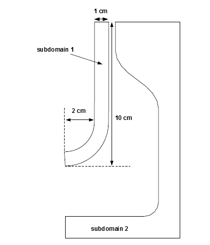
The domain for the problem is divided into two subdomains: one for the fluid preform (subdomain 1) and the other for the mold (subdomain 2). Incompressibility and momentum equations are solved in subdomain 1 (the fluid preform). The problem involves two free surfaces (boundary 2 and boundary 4, shown in Figure 2). boundary 2 will eventually come into contact with the mold, and its position is calculated as a part of the solution.
The fluid preform has a density of  =1 g/cm3 and a viscosity of
  = 100000 poise. Inertia terms and the effects
of gravity will be included in the calculation.
= 100000 poise. Inertia terms and the effects
of gravity will be included in the calculation.
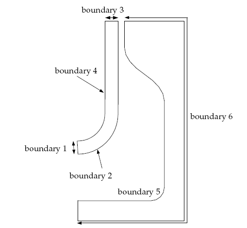
The boundary sets for the problem are shown in Figure 2.2: Boundary Set for the Problem, and the conditions at the boundaries of the domain (for the preform) are:
boundary 1: symmetry axis
boundary 2: free surface
boundary 3: zero normal velocity and zero surface force
boundary 4: free surface
The following sections describe the setup and solution steps for this tutorial:
To prepare for running this tutorial:
Prepare a working folder for your simulation.
Download the
2d_axi_blow_molding.zipfile here .Unzip the
2d_axi_blow_molding.zipfile you have downloaded to your working folder.The mesh file
2d-axi-blowmold.mshcan be found in the unzipped folder.Start Workbench from .
Create a Fluid Flow (Polyflow Classic) analysis system by drag and drop in Workbench.
Save the Ansys Workbench project using File → , entering
Final-blow-moldas the name of the project.Import the mesh file (
2d-axi-blowmold.msh).Double-click the Setup cell to start Polydata.
When Polydata starts, the Create a new task menu item is highlighted, and the geometry for the problem is displayed in the Graphics Display window.
In the following steps you will define a new task representing the 2D axisymmetric time-dependent model. Then, define the mold and a sub-task for the isothermal flow calculation.
Create a task for the model.
 Create a new task
Select the following options:
F.E.M. task
Time-dependent problem(s)
2D axisymmetric geometry
The Current setup is updated to reflect the selected options. This example is a simulation of blow molding for a 2D axisymmetric bottle and the mold is two-dimensional. The problem is assumed to be time-dependent.
Click Accept the current setup.
Define the mold.
Define molds
Create a mold.
Create a new mold
Select an adiabatic mold.
Adiabatic mold
When prompted, click to retain the default name for the mold (Mold 1).
Specify the solid region that represents the mold.
Domain of the mold
Select SUBDOMAIN_1 and click .
SUBDOMAIN_1 is moved from the top list to the bottom list, indicating that the mold is defined as SUBDOMAIN_2 .
Click Upper level menu at the top of the menu.
Specify the boundary that represents the part of the mold that comes into contact with the fluid.
Polyflow Classic uses this information to determine the penetration distance (into the mold) of every point of the free surface (BOUNDARY2).
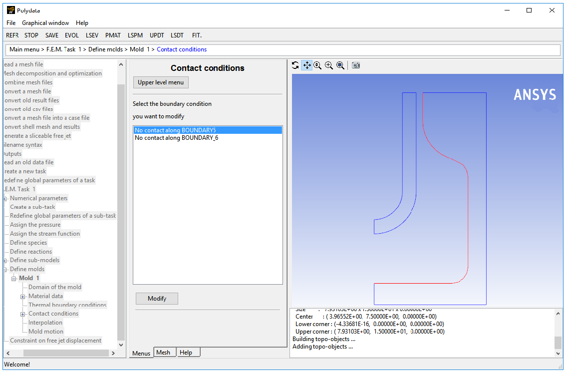
Contact conditions
Select No contact along BOUNDARY5 and click .
The free surface, BOUNDARY2 of the preform comes into contact with the mold wall, BOUNDARY5 (as shown in Figure 2.2: Boundary Set for the Problem).
Select Contact.
Click Upper level menu four times to return to the F.E.M. Task 1 menu.
Create a sub-task for the isothermal flow.
Create a sub-task
Select Generalized Newtonian isothermal flow problem.
A dialog box opens, asking for the title of the problem.
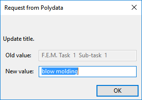
Enter
blow moldingas the New value and click .The Domain of the sub-task menu item is highlighted.
Define the domain where the sub-task applies.
The domain is divided into two subdomains, one for the fluid preform (SUBDOMAIN_1) and the other for the mold (SUBDOMAIN_2). In this problem, the sub-task applies only to the preform.
Domain of the sub-task
Select SUBDOMAIN_2 and click .

SUBDOMAIN_2 is moved from the top list to the bottom list, indicating that the sub-task is defined on SUBDOMAIN_1 .
Click Upper level menu at the top of the menu.
The Material data menu item is highlighted.
Polydata indicates which material properties are relevant for the sub-task by graying out the irrelevant properties. In this case, viscosity, density, inertia terms, and gravity are available for specification.
![]() Material data
Material data
Define the viscosity of the preform.
Click Shear-rate dependence of viscosity.
Click Constant viscosity.
Click Modify fac to specify the value of
 , which is referred to as “fac”
in the graphical user interface.
, which is referred to as “fac”
in the graphical user interface.Polydata prompts for the new value of the viscosity.
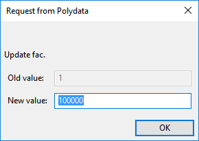
Enter
100000[units: poise] as the New value and click .Click Upper level menu two times to continue with the Material Data specification.
Define the density of the preform.
Click Density.
Click Modification of density to specify the value of the density.
Polydata prompts for the new value of the density.
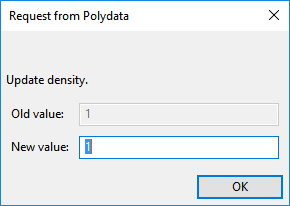
Enter
1[units: g/cm3] as the New value and click .Click Upper level menu to continue with the Material Data specification.
Enable the calculation of the inertia terms in the momentum equation.
In this problem inertia plays an important role. When internal pressure is applied, the preform expands, and the fluid accelerates towards the mold. In order to obtain a realistic blowing time, inertia must be taken into account.
Click Inertia terms.
Select Inertia will be taken into account.
Click Upper level menu to continue with the Material Data specification.
Include the effects of gravity in the flow.
The fluid preform flows in the negative y direction under gravity, so specify the component of gravity along the y direction (
 ).
).
Click Gravity.
Click Modify gy to specify the value of gravity in the y direction.
Modify gy
Polydata prompts for the new value of the gravity along the y-axis.
Enter
-981[units: cm/s2] as the New value and click .Click Upper level menu two times to return to the blow molding menu.
The Flow boundary conditions menu item is highlighted.
In the following steps you will set the conditions at each of the boundaries of the domain. When a boundary set is selected, its location is highlighted in red in the graphics window.
![]() Flow boundary conditions
Flow boundary conditions
Retain the default condition Axis of symmetry along BOUNDARY1.
No action is required to accept the default value. You can simply proceed to the next step. For 2D axisymmetric models, Polydata recognizes the axis of symmetry from the mesh file and automatically imposes the symmetry condition along the line
 .
.
Set the conditions at the outer free surface (BOUNDARY2).
The free surface boundary condition in contact detection problems is different from their simulations in Polyflow Classic. In blow molding problems, a free surface comes into contact with a solid mold. Polyflow Classic applies a contact detection algorithm at each location of the surface to detect the occurrence of the contact.
You need to specify the following for the free surface on BOUNDARY2:
the components of the direction of displacement along BOUNDARY1 and BOUNDARY3
the contact wall (the boundary of the mold along which the contact is detected)
the penalty coefficient
This determines the accuracy of the contact; the smaller its value, the deeper the contact is.
the slipping coefficient
The fluid may slip along the contact wall, so to take this factor into account, a slipping coefficient must be specified along the tangential direction.
Select Zero wall velocity (vn=vs=0) along BOUNDARY2 and click Modify.
Click Free surface.
Specify the contact detection problem.
Click Contact (blow mold).
Click Create a new contact problem.
Specify where the free surface will contact the mold.
Polyflow Classic uses the definition of the contact wall in the determination of the penetration distance (into the mold) of every point of the free surface (BOUNDARY2).
Click Select a contact wall.
Select Mold 1 : Contact along BOUNDARY5 and click .
As shown in Figure 2.2: Boundary Set for the Problem, the free surface (BOUNDARY2) of the preform comes into contact with the mold (BOUNDARY5).
Define the slipping coefficient.
Modify slipping coefficient
Retain the default value of 1e+12 and click .
With such a high value of the slipping coefficient, the fluid will stick to the contact wall.
Define the penalty coefficient.
Modify penalty coefficient
Retain the default value of 1e+12 and click .
Click Upper level menu two times to return to the Kinematic condition menu.
Click Upper level menu to return to the Flow boundary conditions panel.
In contact detection problems, abrupt changes in the velocity field occur at the contact points between the fluid preform and the mold. Polydata gives the warning message shown below. Since the prediction of the velocity field in such cases destroys the prediction scheme, you can continue by clicking .
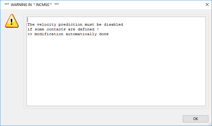
Click to accept the warning and continue.
Set the conditions at the top part of the preform (BOUNDARY3).
Select Zero wall velocity (vn=vs=0) along BOUNDARY3 and click Modify.
Click Normal velocity and tangential force imposed ( vn, fs ).
Click Upper level menu to accept the default value of 0 for the normal velocity,
 .
.Click Upper level menu to accept the default value of 0 for the tangential force,
 .
.
Set the conditions at the inner free surface (BOUNDARY4).
This boundary of the preform is subjected to pressure by the application of a normal force, so specify a normal force along this boundary.
Select Zero wall velocity (vn=vs=0) along BOUNDARY4 and click Modify.
Click Free surface.
Specify the normal force.
Click Normal force.
Select Constant.
Polydata prompts for the new value of the normal force.
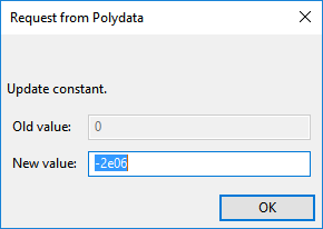
Enter
-2e06as the New value and click .Click Upper level menu.
Click Upper level menu to return to the Flow boundary conditions menu.
Click Upper level menu to return to the blow molding menu.
The Global remeshing menu item is highlighted.
This model involves free surfaces for which the positions are unknown. A portion of the mesh is affected by the relocation of these boundaries. Hence a remeshing technique is applied on this part of the mesh. The free surfaces are entirely contained within SUBDOMAIN_1, and hence only SUBDOMAIN_1 is affected by the relocation of the free surfaces.
![]() Global remeshing
Global remeshing
Specify the region where the remeshing is to be performed (SUBDOMAIN_1).
1–st local remeshing
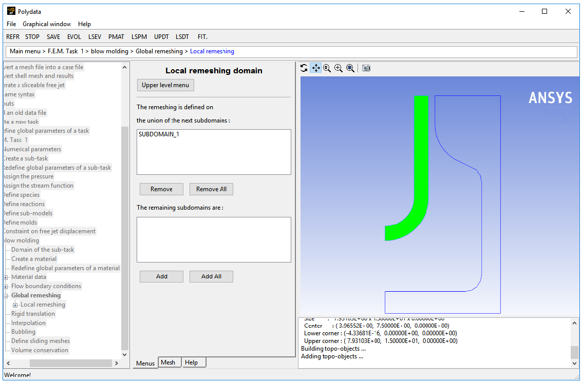
Click Upper level menu to accept the default selection of SUBDOMAIN_1.
Click Lagrangian on the border only.
For information on remeshing techniques, see Appendix.
Click Accept the current setup in the Element distortion check menu.
In blow molding simulations, the finite-element mesh can undergo great deformations. The Element distortion check menu deals with the detection of all possible distortions of the elements. In this problem, you can accept the default options and proceed to the next step.
Click Upper level menu two times to return to the F.E.M. Task 1 menu.
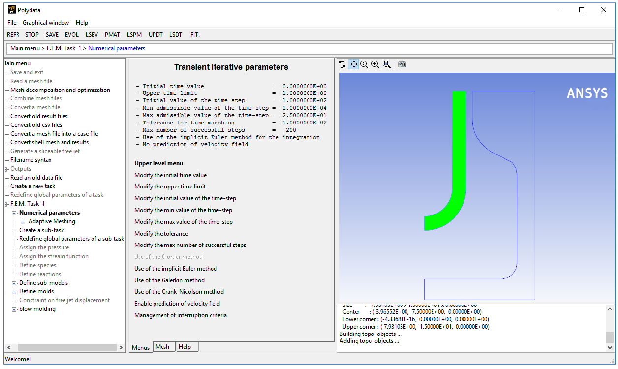
In the following steps you will define the numerical parameters for the simulation.
![]() Numerical parameters
Numerical parameters
Specify the parameters for the iterative scheme in the calculation of the free surface.
Modify the transient iterative
parameters
For information on time marching scheme, see Appendix.
Specify the time limit.
This option specifies the time at which the solution procedure stops.
Modify the upper time limit
Polydata prompts for the new value of the time limit.
Enter
0.1[units: s] as the New value and click .Specify the initial value of the time step.
This option is used to define the initial time step, which is used for the calculation of the next two time steps. After that, the step size is automatically calculated by Polyflow Classic. This first time step should be set according to the characteristic time scale of the process considered.
Modify the initial value
of the time-step
Enter
1e-03[units: s] as the New value and click .Specify the minimum value for the time step.
If a calculated value for the time step falls below the minimum for the time step at any point in the calculation, the iterative scheme stops since this might be a symptom of calculation difficulties.
Modify the min value of the time-step
Enter
1e-07[units: s] as the New value and click .Specify the maximum value for the time step.
In order to guarantee accuracy of the time-marching scheme and to avoid useless calculations (rejection of inaccurate time steps), you can limit the growth of the time increment.
Modify the max value of the time-step
Enter
1e-03[units: s] as the New value and click .Specify the tolerance for time marching.
The tolerance is the admissible error between the predicted solution and the exact solution at a particular time step. A very small value of the tolerance can result in large computational costs and a very large value can result in wrong solution.
Modify the tolerance
Retain the default value of 0.01 and click .
Specify the maximum number of successful steps.
This option is used to select the maximum number of converged steps. If this value is reached, the calculation stops, even if the upper time limit has not been reached.
Modify the max number
of successful steps
Retain the default value of 200 and click .
Enable Use of the implicit Euler method.
Click Upper level menu three times to return to the top-level Polydata menu.
You can specify how often Polyflow Classic saves the solution data when it calculates a solution. In this tutorial, save the results at every 4 time steps.
![]() Outputs
Outputs
Click Output Triggering.
Click Enter the number of steps.
Polydata prompts you for the number of steps.
Enter
4as the New value and click .
Click Upper level menu twice.
Specify the system of units.
Click Modify system of units.
Click Set to metric_cm/g/s/A+Celsius.
Click Upper level menu twice to return to the top-level Polydata menu.
In the following steps you will create a postprocessor sub-task to compute the thickness of the blown product. The results of this postprocessor are sent to CFD-Post as a value field.
![]() F.E.M. Task 1
F.E.M. Task 1
Create a new sub-task.
Create a sub-task
Click when asked whether you want to copy an existing sub-task.
Click Postprocessor.
Enter
parison thicknessas the New value for the title and click .
Click Parison thickness.
Click parison #01.
Click twice to accept the warnings about defining the borders.
You will have to define these borders at a later stage.
Specify the region where the postprocessor sub-task applies.
Domain of the sub-task
Accept the default of SUBDOMAIN_1 by clicking Upper level menu.
Specify the boundary sets representing the starting and ending borders to be used in the thickness calculation.
Polyflow Classic evaluates the distance between these borders at a point between them to determine the thickness at that location.
Borders for thickness calculation
Select BOUNDARY2: not used and click .
Click Starting border.
Select BOUNDARY4: not used and click .
Click Ending border.
Click Upper level menu five times to return to the top-level Polydata menu.
![]() Save and exit
Save and exit
Polydata asks you to confirm fields that are to be saved to the results file for postprocessing.
Click Accept.
This confirms that the default Current field(s) are correct.
Click Continue.
This accepts the default names for graphical output files (
cfx.res) that are to be saved for postprocessing, and the Polyflow Classic format results file is (res).
In the following steps you will run Polyflow Classic to calculate a solution for the model you just defined using Polydata.
Run Polyflow Classic by right-clicking the Solution cell of the simulation and selecting .
This executes Polyflow Classic using the data file as standard input, and writes information about the problem description, calculations, and convergence to a listing file (
polyflow.lst).Check for convergence in the listing file.
Right-click the Solution cell and select Listing Viewer....
Workbench opens the View listing file dialog box, which displays the listing file.
It is a common practice to confirm that the solution proceeded as expected by looking for the following printed at the bottom of the listing file:
The computation succeeded.
Use CFD-Post to view the results of the Polyflow Classic simulation.
Double-click the cell in the Workbench analysis system.
CFD-Post reads the solution fields that were saved to the results file.
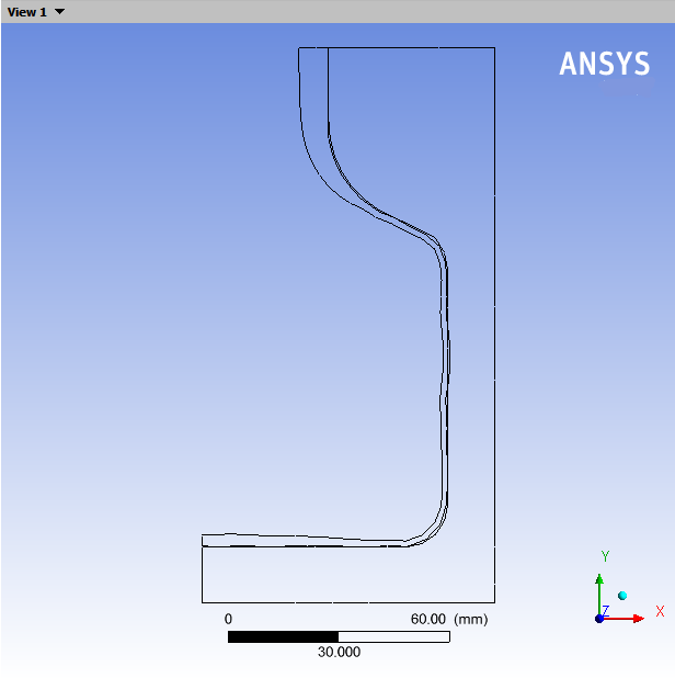
Align the view as shown in the following figure.
Display contours of thickness in the fluid region (SUBDOMAIN_1).
Click the Insert menu and select Contour or click the
 button.
In the box that opens, click to accept the default name (Contour 1) and display the details below the Outline tree.
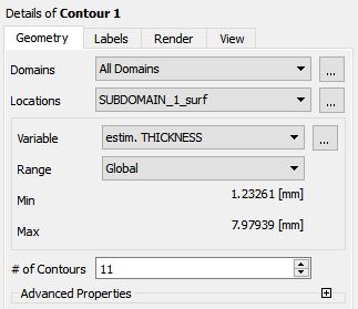
Specify the following settings under the Geometry tab:
Select SUBDOMAIN_1_surf from the Locations drop-down list.
Select estim. THICKNESS from the Variable drop-down list, or click the ellipsis button (
 ) on the right and select estim. THICKNESS.
Click .
Annotate the display.
Click the Insert menu and select Text or click the
 button.
Click to accept the default name (Text 1) and display the details view below the Outline tab.
Enable Embed Auto Annotation under the Definition tab.
Select Time Value from the Type drop-down list.
Click .
Show contours of thickness on the full blown bottle.
Double-click Default Transform in the Outline tree tab, under User Locations and Plots (or right-click Default Transform and select Edit).
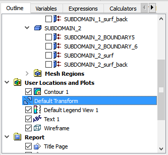
Disable Instancing Info From Domain under the Definition tab in the details of Default Transform.
Enable Apply Reflection, and select YZ Plane from the Method drop-down list.
Retain the default value of 0.0 m for X.
Click .
Click the
 button to center the view.
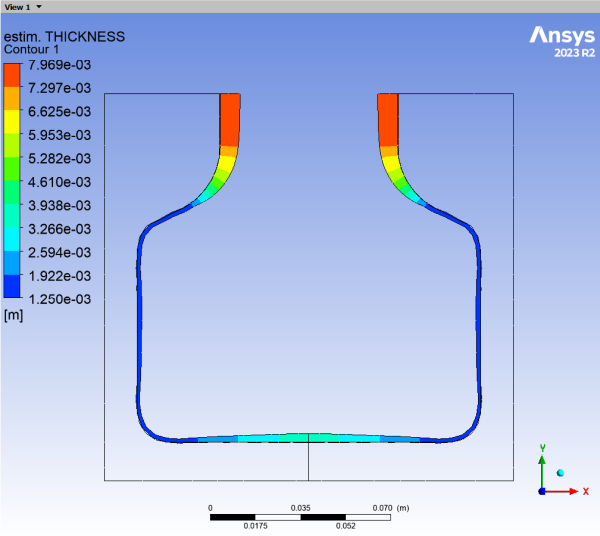
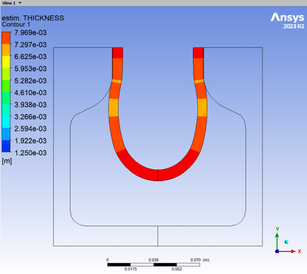
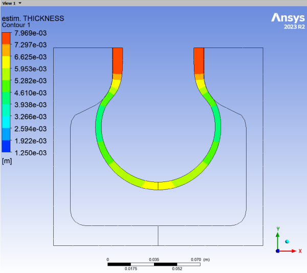
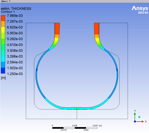
Display contours of thickness at various timesteps.
Display the results at several time steps to see the shape and thickness of the parison during the blow molding process.
Tools → Timestep Selector or click the
 button.
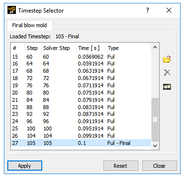
Select the 20 th timestep and click .
Select the 40 th timestep and click .
Select the 60 th timestep and click .
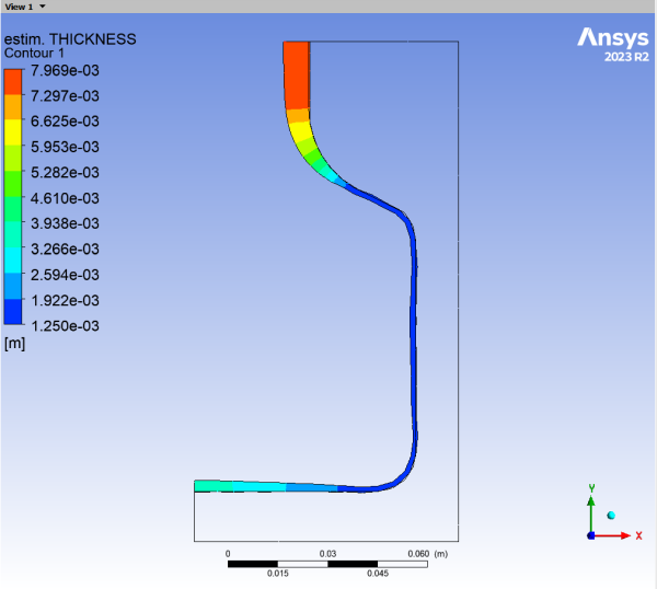
Select the final timestep and click .
The thickness decreases as the parison inflates. At the final time step, the thickness is smallest where the parison has been the most extended, (in the corner of the bottle). It is largest at the top where the deformation was much less important due to the small diameter here.
Create and save an animation.
Click the Tools menu and select Animation or click the
 button.
Enable Timestep Animation in the Animation dialog box.
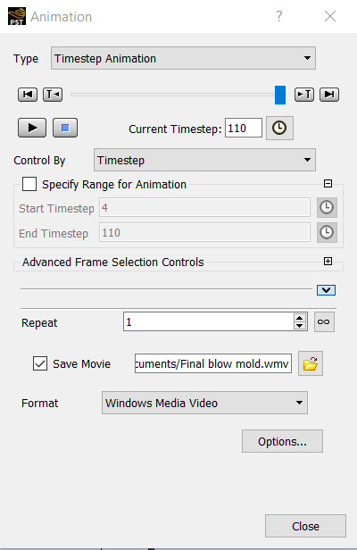
Enable Save Movie to save the animation as a file.
Disable
 to save only one cycle of animations.
Click the start button
 .
.
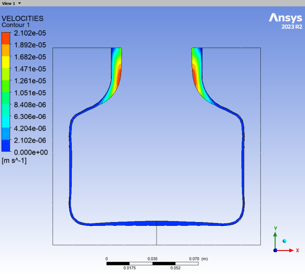
Display contours of velocity in the fluid region.
Double-click Contour 1 under the Outline tab to display the details view.
Select VELOCITIES from the Variable drop-down list and click .
There is zero velocity at the contact between the parison and the mold, but the velocity magnitude is still important where the fluid does not yet touch the mold. At the final time of the simulation, the velocity is near zero, which indicates that the contact is completed. The residual value originates from the penalty formulation used for the contact, as explained in 3D Thermoforming of a Blister.
This tutorial introduced a time-dependent problem with a 2D axisymmetric geometry for the mold. Suitable assumptions were made regarding the nature of the preform and the operating conditions. You analyzed the factors affecting the process in the postprocessing section. An optimization of the preform shape could be performed in order to minimize the weight of the bottle while avoiding weak (too thin) bottle walls.
You used a remeshing method that is most suited for contact detection problems. This problem also introduced the concept of the calculation of free surfaces for contact detection problems. You used efficient numerical techniques to more accurately solve a time-dependent problem.
The appendix covers the following topics:
The purpose of the remeshing technique is to relocate internal nodes according to the displacement of the boundary nodes due to the motion of the free surface. In blow molding applications, the finite-element mesh undergoes large deformations, especially extension. When a thin fluid region is considered, the shear component is essentially absent from the flow kinematics.
Because this application involves contact occurring over time, a Lagrangian representation is used for the free surface that undergoes the contact; this improves the robustness of the contact algorithm. The Lagrangian on the border only technique remeshes based on the combination of a Lagrangian representation on the border of the fluid domain and a minimum-pseudo-energy representation for the inner mesh nodes. For additional information on this technique, see Lagrangian method on borders in the Polyflow Classic User's Guide.
Since this problem is time-dependent, parameters such as flow rate, boundary conditions, or material data are time-dependent. In such problems, the solution of the partial differential equations has to be satisfied at a discrete set of times starting from an initial time. The solution of the equations is obtained by specific integration methods known as predictor-corrector methods. The predictor method calculates a first guess of the solution at a specific time step. This guess is then used by the corrector method to compute the real solution at the time step considered. The data for the time marching scheme is provided in this menu.