


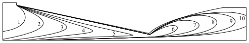
Consider a simple steady-state free surface flow, where the flow enters from the upper left part of the domain. Assuming that the residence time distribution is zero in the entry section, Ansys Polyflow Classic will calculate the residence time distribution in the domain. An example of contour lines of the residence time distribution is shown in Figure 29.1: Contour: Residence Time Distribution for a Steady-State Free Surface Problem.
Ansys Polyflow Classic computes the residence time distribution using the equation
 | (29–3) |
where  at time
  , and the boundary conditions along the entry sections are taken
into account.
, and the boundary conditions along the entry sections are taken
into account.  is the residence time, and
  is the material derivative of the residence time.
Equation 29–3 states that
the residence time increases as the absolute time  for particles along their path increases. It is a hyperbolic
equation, and it requires boundary conditions (as well as initial conditions for
time-dependent problems). The value of the residence time must be set along all
entry sections.
for particles along their path increases. It is a hyperbolic
equation, and it requires boundary conditions (as well as initial conditions for
time-dependent problems). The value of the residence time must be set along all
entry sections.
Usually you will set a value of zero. On all sections on which an inflow boundary condition has been applied for the momentum equation, the residence time is set to zero by default. You can add boundary conditions on entry sections where a different type of condition has been selected.
For time-dependent calculations, Ansys Polyflow Classic imposes  as an initial condition. In this case, the time-dependent problem
is well-posed provided that
as an initial condition. In this case, the time-dependent problem
is well-posed provided that  has been imposed on all entry sections. For steady-state problems,
Equation 29–3 does not
define a well-posed problem in recirculating zones (vortices) and along walls where
has been imposed on all entry sections. For steady-state problems,
Equation 29–3 does not
define a well-posed problem in recirculating zones (vortices) and along walls where
 .
.
This is not usually important, since the residence time distribution is meaningless in these regions, and you can easily exclude these corresponding contour lines from the display in your graphical postprocessing program. In Figure 29.1: Contour: Residence Time Distribution for a Steady-State Free Surface Problem, contour lines have been selected such as to eliminate large numbers of contours along walls.
Another possibility for calculating the residence time distribution in the
presence of steady-state vortices is to define a time-dependent problem that uses a
steady-state velocity field that has already been calculated. In this cases, the
velocity field will be obtained from the res file.
The residence time distribution postprocessor uses the 4×4 subelement technique in 2D and the 2×2×2 subelement technique in 3D, together with a consistent streamline-upwinding/Petrov-Galerkin formulation.
While the residence time distribution is calculated for most flow problems, this option is not available when sliding meshes are defined.