


The transformation maps a parent domain into a deformed domain. The transformation
begins with the construction of a global coordinate system, defined on a simply
shaped domain. These global coordinates represent a mapping of the
irregularly-shaped computational domain into a regular parent domain (such as a
square in 2D or a cube in 3D). For example, the irregular domain shown in Figure 15.3: Thompson Transformation is
mapped onto a square by the global-coordinates transformation function
 . The coordinates
  have the same number of components as the mesh coordinates
 .
.
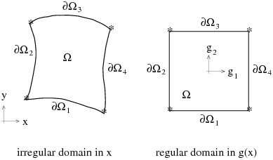
In the 2D case shown in Figure 15.3: Thompson Transformation,
the global coordinates  are constructed on the basis of the following equation:
 | (15–6) |
with the following boundary conditions:
 | (15–7) |
The Thompson transformation for this example is simply the inverse mapping
 . Once
  has been constructed, the Thompson transformation is the solution
 that satisfies Equation 15–6
with appropriate boundary conditions. The calculation of the
that satisfies Equation 15–6
with appropriate boundary conditions. The calculation of the  field, as well as the Thompson transformation itself, is solved by
standard finite-element techniques.
field, as well as the Thompson transformation itself, is solved by
standard finite-element techniques.
Equation 15–6
is linear in  , but not in
  . The Thompson transformation is inherently nonlinear in
 , even though the Laplacian is a linear operator. The construction
of the
, even though the Laplacian is a linear operator. The construction
of the  field is performed only once at the beginning of the simulation,
before the main solver starts. The Thompson transformation is then solved in a
coupled fashion, together with the equations governing the flow.
field is performed only once at the beginning of the simulation,
before the main solver starts. The Thompson transformation is then solved in a
coupled fashion, together with the equations governing the flow.
The choice of boundary conditions given to  and
and  in the Thompson transformation governs the remeshing itself. The
Thompson transformation is applied to the remeshing subdomain. Each separate
sub-boundary of the remeshing subdomain is referred to as a segment. On each
segment, one component of the vector
in the Thompson transformation governs the remeshing itself. The
Thompson transformation is applied to the remeshing subdomain. Each separate
sub-boundary of the remeshing subdomain is referred to as a segment. On each
segment, one component of the vector  (essential boundary condition) must be specified, while a
zero-normal-derivative condition (natural boundary condition) is applied to the
other component(s).
(essential boundary condition) must be specified, while a
zero-normal-derivative condition (natural boundary condition) is applied to the
other component(s).