


The Material is used to calculate mass and mass moment of inertia of a body such as a Rigid body, Nodal FE Body, Nodal EasyFlex Body, or Beam Group.
The Material is also used to calculate an internal force for a finite element, EasyFlex element and beam group. Motion solver supports linear elastic, hyper elastic, foam, and plastic materials.
The density ρ of the material is used to calculate mass and mass moment of inertia at the center of mass of the body reference frame as follows.
 | (7–272) |
 | (7–273) |
where:
| M = mass of the body |
| ρ = density of the body |
| V = volume of the body |
| s′ = displacement of a mass particle from the center of mass in the body reference frame |
The internal force of fe a finite element and EasyFlex element can be taken from the partial derivatives of the strain energy for the deformation of u as follows.
 | (7–274) |
where:
| U = strain energy of the elements |
The strain energy will be introduced in each formulation of the material.
Linear materials have three possible models:
ISOTROPIC, LINEAR THERMAL
ISOTROPIC, NONLINEAR THERMAL
ORTHOTROPIC, LINEAR
For orthotropic material, thermal material cannot be applied.
Strain energy of the elements and can be written as:
 | (7–275) |
where:
 = =  = elastic strain vector = elastic strain vector |
 = total strain vector = = total strain vector =  |
 = thermal strain vector defined in Equation 7.18 = thermal strain vector defined in Equation 7.18 |
 = stress vector = = stress vector =  |
 = stress-strain relationship matrix (constitutive
matrix) = stress-strain relationship matrix (constitutive
matrix) |
The stress is related to the strains by:
 | (7–276) |
In Equation 7–275, the stress-strain relationship of the isotropic model can be written using strain tensor as follows:
 | (7–277) |
where:
| E = Young's modulu |
| G = shear modulus |
| v = Poisson's ratio |
| λ = lame modulus and is: |
 | (7–278) |
From Equation 7–277, the stress-strain relationship of the isotropic model can be rewritten in the matrix form:
 | (7–279) |
This may also be inverted to:
 | (7–280) |
 | (7–281) |
where:
| D-1 = compliance matrix |
The table below shows representative values for densities and elastic constants for the major isotropic materials.
Figure 7.34: Major Isotropic Materials
| Material | Density (1e-6 kg/mm³) | Young's Modulus (1e+3 MPa) | Poisson's Ratio |
| Tungsten Carbide | 14 ~ 17 | 450 ~ 650 | 0.22 |
| Silicon Carbide | 2.5 ~ 3.2 | 450 | 0.15 |
| Tungsten | 13.4 | 410 | 0.30 |
| Alumina | 3.9 | 390 | 0.25 |
| Titanium Carbide | 4.9 | 380 | 0.19 |
| Silicon Nitride | 3.2 | 270 ~ 320 | 0.22 |
| Nickel | 8.9 | 215 | 0.31 |
| CFRP Laminate | 1.5 ~ 1.6 | 70 ~ 200 | 0.20 |
| Iron | 7.9 | 196 | 0.30 |
| Low Alloy Steels | 7.8 | 200 ~ 210 | 0.30 |
| Stainless Steel | 7.5 ~ 7.7 | 190 ~ 200 | 0.30 |
| Mild Steel | 7.8 | 196 | 0.30 |
| Copper | 8.9 | 124 | 0.34 |
| Titanium | 4.5 | 116 | 0.30 |
| Silicon | 2.5 ~ 3.2 | 107 | 0.22 |
| Silica Glass | 2.6 | 94 | 0.16 |
| Aluminum & Alloys | 2.6 ~ 2.9 | 69 ~ 79 | 0.35 |
| Concrete | 2.4 ~ 2.5 | 45 ~ 50 | 0.1 ~ 0.2 |
| GFRP Laminate | 1.4 ~ 2.2 | 7 ~ 45 | 0.28 |
| Wood, Parallel Grain | 0.4 ~ 0.8 | 9 ~ 16 | 0.2 |
| Polyamides | 1.4 | 3 ~ 5 | 0.1 ~ 0.45 |
| Nylon | 1.1 ~ 1.2 | 2 ~ 4 | 0.25 |
| PMMA | 1.2 | 3.4 | 0.35 ~ 0.4 |
| Polycarbonate | 1.2 ~ 1.3 | 2.6 | 0.36 |
| Natural Rubbers | 0.83 ~ 0.91 | 0.01 ~ 0.1 | 0.49 |
| PVC | 1.3 ~ 1.6 | 1.5 | 0.41 |
From Equation 7–275 to Equation 7–277, the stress-strain relationship of the orthotropic model can be rewritten in the matrix form:
 | (7–282) |
where typical terms are:
| Ex = Young's modulus in x-direction |
| vxy = xy-Poisson's ratio |
| Gxy = xy-Shear modulus |
| Δ = determinant of the compliance matrix D-1 and is: |
 | (7–283) |
The parameters vyx, vyz and vxz must be defined by the user. The D-1 matrix is presumed to be symmetric, the values of vyx, vzx and vzy are calculated as:
 | (7–284) |
 | (7–285) |
 | (7–286) |
Note: The Poisson's ratio is typically valid in the range of 0≤v≤0.5. Be aware that if the calculated vyx, vzx and vzy by Equation 7–284 to Equation 7–286 exceed this valid range, the Motion solver will output a warning message and may show unexpected solutions.
Thermal materials exhibit changes in shape, area, and volume in response to temperature variations. Properties such as the coefficient of thermal expansion, thermal conductivity, specific heat, and reference temperature are crucial for calculating the nodal temperature and resulting thermal strain from heat transfer.
Thermal materials are classified based on their behavior under temperature changes into two main categories: linear thermal materials and non-linear thermal materials.
Linear thermal materials are characterized by their constant thermal properties over a significant range of temperatures.
The primary properties include:
Coefficient of Thermal Expansion (α): This measures how much a material expands per unit change in temperature, typically remaining constant for linear materials. The coefficient is applied in all directions of an element. The formula is given by:
 | (7–287) |
where:
| L = original length |
 = rate of change in length per unit change in
temperature = rate of change in length per unit change in
temperature |
Thermal Strain (εth): As the material undergoes a temperature change, it experiences a thermal strain, calculated by:
 | (7–288) |
where:
| ΔT = change in temperature from the reference temperature |
Thermal Conductivity (k): It quantifies the material's ability to conduct heat, expressed as:
 | (7–289) |
where:
| q = heat flux |
| k = thermal conductivity |
| ∇T = temperature gradient |
Specific Heat (c): This property indicates the amount of heat per unit mass required to raise the unit temperature and is defined as:
 | (7–290) |
where:
| C = heat capacity |
| ρ = density |
| V = volume of a body |
The reference temperature is typically set based on the material’s application, providing a baseline for thermal expansion and other calculations.
The above thermal properties are used to construct the governing equation for Thermal Analysis.
Non-linear thermal materials are characterized by properties that change with temperature. Unlike linear materials, where properties such as Young's modulus E, the coefficient of thermal expansion α, thermal conductivity k, and specific heat c are constant, non-linear materials require these properties to be defined as functions of temperature such as E(T), α(T), k(T), and c(T), typically provided in the form of temperature-value curves. The thermal strain εth is calculated by the formula:
 | (7–291) |
where:
| α(T) = coefficient of thermal expansion as a function of temperature T |
Note: In the input data, the x-axis represents temperature, and the y-axis represents the values of each parameter dependent on temperature.
Hyperelasticity refers to a constitutive response derivable from an elastic free-energy potential. It is typically used for materials experiencing large elastic deformation. Applications for elastomers such as vulcanized rubber and synthetic polymers, along with some biological materials, often fall into this category.
The microstructure of polymer solids consists of chain-like molecules. The flexibility of the molecules allows for an irregular molecular arrangement, leading to complex behavior. Polymers are usually isotropic at small deformation and anisotropic at larger deformation, as the molecule chains realign to the loading direction. Under an essentially monotonic loading condition, however, many polymer materials can be approximated as isotropic.
Some classes of hyperelastic materials cannot be modeled as isotropic, such as:
Fiber-reinforced polymer composites. Typical fiber patterns include unidirectional and bidirectional, and the fibers can have a stiffness that is 50-1000 times that of the polymer matrix, resulting in a strongly anisotropic material behavior.
Biomaterials (such as muscles and arteries). These anisotropic materials can experience large deformation in which the anisotropic behavior is due to their fibrous structure.
The typical volumetric behavior of hyperelastic materials can be grouped into two classes:
Materials typically having small volumetric changes during deformation, such as polymers. These are incompressible or nearly-incompressible materials.
Materials having large volumetric changes during deformation, such as foams. These are compressible materials. For more information, See Foam Materials.
The Motion solver supports four incompressible isotropic hyper elastic models, Neo-Hookean, Arruda-Boyce, Ogden and Mooney-Rivlin. These models are classified as Incompressible or nearly-incompressible isotropic models.
For each hyperelastic material, you must define a material incompressibility parameter D. This parameter determines the penalty of a volume constraint. The smaller the value, the tighter the volume constraint. When a flexible body with a hyperelastic material is in contact with the other body, the motion solver sometimes has a small step size. In this case, increasing this value can increase the step size.
The form Neo-Hookean strain-energy potential is:
 | (7–292) |
where:
| C10 = material constant |
| D = material incompressibility parameter |
| J = volume strain |
| Ii = principal invariants of the left Cauchy-Green deformation tensor |
 = modified invariants, calculated as: = modified invariants, calculated as: |
 | (7–293) |
The relationship between initial shear modulus μ0 and C10 is:
 | (7–294) |
where:
| μ0 = initial shear modulus |
The initial bulk modulus is related to the material incompressibility parameter by:
 | (7–295) |
where:
| K = initial bulk modulus |
The form of the strain-energy potential for Arruda-Boyce model is:
 | (7–296) |
where:
| μ = initial shear modulus of material |
| λM = limiting network stretch (locking stretch) |
| D = material incompressibility parameter |
| J = volume strain |
| = first
invariant of Cauchy-Green deformation tensor |
The Ogden form of strain-energy potential is based on the principal stretches of left-Cauchy strain tensor, which has the form:
 | (7–297) |
where:
| n = the number of terms in the summation of the Ogden model |
| μk, αk and Dk = material constants |
 = deviatoric principal stretches at the
ith principal axis which can be calculated with the
eigenvalue of the Cauchy-Green deformation tensor of
λi as follows: = deviatoric principal stretches at the
ith principal axis which can be calculated with the
eigenvalue of the Cauchy-Green deformation tensor of
λi as follows: |
 | (7–298) |
The initial shear modulus, μ is given as:
 | (7–299) |
The initial bulk modulus K is defined by:
 | (7–300) |
Remarks
The strain-energy potential of the Ogden compressible foam model defined in the MAPDL solver is:
 | (7–301) |
where:
 and and  = material constants (user input values in the Engineering
Data of Ansys Workbench) = material constants (user input values in the Engineering
Data of Ansys Workbench) |
In the form of the above formula, the following relationship is established:
The Motion solver only supports two-term Mooney-Rivlin model. The form of the strain energy potential for a two-parameter Mooney-Rivlin model is:
 | (7–302) |
where:
| C10 and C01 = material constants |
| D = material incompressibility parameter (user input) |
| J = volume strain |
 = first invariant of Cauchy-Green deformation tensor = first invariant of Cauchy-Green deformation tensor |
 = second invariant of Cauchy-Green deformation tensor = second invariant of Cauchy-Green deformation tensor
|
The initial shear modulus is given by:
 | (7–303) |
where:
| μ = initial shear modulus |
The initial bulk modulus is:
 | (7–304) |
where:
| K = initial bulk modulus |
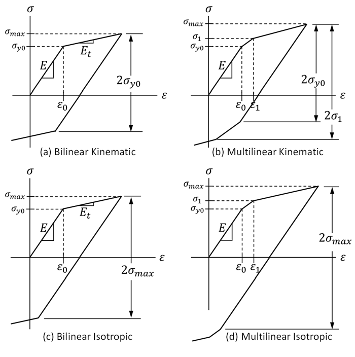
Plasticity materials encompass substances capable of enduring permanent deformation under load, a critical aspect in engineering applications requiring durability beyond elastic limits. Ansys Motion supports two principal plasticity models: BILINEAR and MULTILINEAR, which cater to varying degrees of material stress responses as depicted in their respective strain-stress curves. These models are essential for simulating conditions under which materials yield or harden, accommodating changes in yield surfaces that dictate the subsequent yielding conditions through isotropic and kinematic hardening rules.
The nominal strain-stress curves for BILINEAR and MULTILINEAR models are shown in the figure below:
where:
| σy0 = initial yielding stress |
| E = Young's modulus for linear material |
| Et = tangent modulus |
If the nominal stress is equal to an initial yielding stress σy0, the material will develop plastic strains. If it is less than σy0, the material is elastic and the stresses will develop according to the elastic stress-strain relations and the formulation of the material is identical to that of a linear material. The strain-stress relationship in the plastic region is defined by tangent modulus Et. For tangent modulus, as this value becomes zero, the material is close to the perfect plasticity. In this case, the Motion solver will more iterate to find the yielding stress.
Note: When using the Motion Standalone Preprocessor for multilinear plasticity materials, the strain-stress relationship in the plastic region is defined by a spline. The x-axis of the spline represents the differences in strain, Δε, and the y-axis represents the nominal stress, σi as shown in Figure 7.5: Definition of Multilinear Strain-Stress Curve for Motion Standalone Preprocessor. The differences in strain, Δεi, are defined as:
 | (7–305) |
where:
| εi = ith nominal strain in the nominal strain-stress curve |
| n = total amount of data for the multilinear plasticity material |
When using Workbench environment, Strain-Stress curves defined in the Engineering Data are automatically converted to Δεi and σi and written to the solver input file.
Figure 7.36: Definition of Multilinear Strain-Stress Curve for Motion Standalone Preprocessor
| No. | X-Data (Δεi) | Y-Data (σi) |
| 1 | ε1 - ε0 | σ1 |
| 2 | ε2 - ε0 | σ2 |
| 3 | ε3 - ε0 | σ3 |
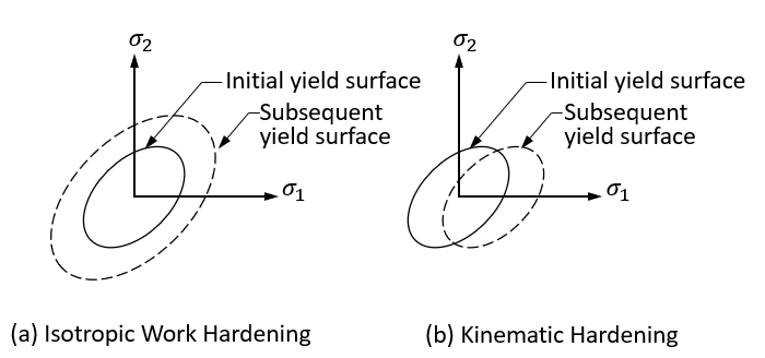
The hardening rule describes the changing of the yield surface with progressive yielding, so that the conditions (stress states) for subsequent yielding can be established. Two hardening rules are available: work (or isotropic) hardening and kinematic hardening. In work hardening, the yield surface remains centered about its initial center line and expands in size as the plastic strains develop. For materials with isotropic plastic behavior this is termed isotropic hardening and is shown in Figure 7.37: Types of Hardening Rules (a). Kinematic hardening assumes that the yield surface remains constant in size and the surface translates in stress space with progressive yielding, as shown in Figure 7.37: Types of Hardening Rules (b).
Motion support two types of linear kinematic hardening: Beta (β) and Prager linear hardening.
The total strain is defined as:
 | (7–306) |
where:
| εt = total strain |
| εe = elastic strain |
| εp = plastic strain |
The option for Plastic Strain in the analysis setting determines whether to calculate the total strain as true strain or as engineering strain.
The plastic hardening modulus is calculated from the following equation.
 | (7–307) |
where:
| Ep = plastic hardening modulus |
The yielding stress and plastic strain can be calculated as the unknown variables in the Motion solver.
The Cauchy stress of the plasticity material can be expressed using stretch as follows:
 | (7–308) |
where:
| τ = nominal stress |
| λ = nominal stretch |
The nominal stress can be calculated with the strain as follows:
 | (7–309) |
where f(εi) can be determined from the strain-stress curve.
Beta (β) is a model that linearly represents the fundamental concepts of isotropic hardening, kinematic hardening, and combined hardening, which is an intermediate state between the two. The hardening rule according to the value of β is as follows:
 | (7–310) |
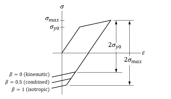
The corresponding yield stress can be defined as follows, increasing with plastic deformation:
 | (7–311) |
For a more detailed explanation of isotropic hardening and kinematic hardening, refer to Isotropic Hardening and Kinematic Hardening in the Material Reference.
The Prager linear hardening model is a specific case of the Chaboche kinematic hardening model. The Chaboche model is an advanced plasticity model that accounts for both isotropic and kinematic hardening through a series of nonlinear equations. The model's general form can be expressed as follows:
 | (7–312) |
where:
| x = back stress |
| ci, γi, i = 1,2,…,n = material constraints for kinematic hardening |
The back stress x is superposition of several kinematic models as:
 | (7–313) |
where:
| n = number of kinematic models to be superposed |
In Prager linear hardening, γ is assumed to be 0, and the number of kinematic models is 1. Thus:
(7–314) |
or equivalently,
 | (7–315) |
For a more detailed explanation of Chaboche kinematic hardening, refer to Nonlinear Kinematic Hardening in the Material Reference.
Remarks
To obtain the same solution as when β=1 using the Prager linear hardening model, use c and E_t as follows:
 | (7–316) |
 | (7–317) |
where:
 = value corresponding to
Et when Beta is used for the
linear kinematic hardening type = value corresponding to
Et when Beta is used for the
linear kinematic hardening type |
To obtain the same solution as when β=0 using the Prager linear hardening model, use c and Et as follows:
 | (7–318) |
 | (7–319) |
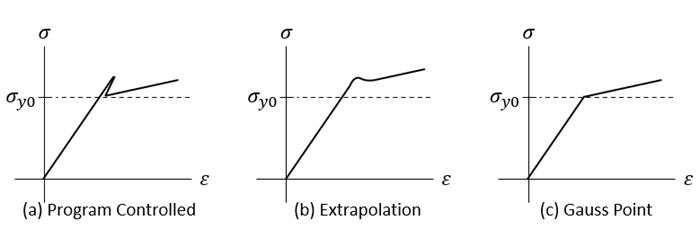
When using plasticity materials, the determination of whether the stress has exceeded the yield stress is evaluated at the element's integration points. If the stress calculated at the Gauss points is extrapolated to the nodal points, the nodal stress may be calculated to be higher than that at the Gauss points. This could cause confusion by suggesting that the material has begun to undergo plastic deformation at points where the nodal stress significantly exceeds the yield stress.
To avoid this confusion, the Motion solver provides the following three options:
(default): If the element is fully elastic, extrapolate the integration-point results to the nodes. If any portion of the element is plastic, copy the integration-point results to the nodes. (Corresponds to the MAPDL Command ERESX,DEFA)
: Extrapolate the linear portion of the integration-point results to the nodes and copy the nonlinear portion (for example, plastic strains). (Corresponds to the MAPDL Command ERESX,YES). For more information on the extrapolation of strain and stress, see the Strain-Stress Extrapolation.
: Copy the integration-point results to the nodes. (Corresponds to the MAPDL Command ERESX,NO)
A foam material is a substance formed by trapping pockets of gas in a solid. The most common examples of foams are sponges and Styrofoam. Foams have a large volume of gas and thin films of solid separating the regions of gas.
A foam material has one model, LOW DENSITY FOAM. The principal stress can be calculated from the principal strain as follows:
 | (7–320) |
where:
| σi = ith principal stress |
| εi = ith principal strain |
| E = Young's Modulus for tension |
| Et = nominal strain-stress spline function for tension defined from user input data |
Poisson's ratio is treated as 0 for a flexible body using a foam material.
Note: For Et, the x-axis represents nominal strain, and the y-axis represents the nominal stress as a function of nominal strain.