


Finite Elements (FE) are an integral part of computational mechanics and are used extensively in simulations involving complex geometries and material behavior under various loading conditions. Finite Element Analysis (FEA) simplifies a complex object by breaking it down into smaller, more manageable elements, making it easier to analyze mechanical stresses and deformations. Finite elements translate the continuum of a mechanical system into a discrete system of elements and nodes.
This chapter begins with an overview of the supported elements, such as beams, shells, and solids, and then details specific elements, discussing their ideal uses, configurations in motion simulations, and how they contribute to strain-stress analysis and elastic force calculations. This structured approach helps you understand how to efficiently use FEA to derive accurate simulations that reflect real-world phenomena.
A Finite Element defines the mass and elastic properties of a nodal FE body. The element is defined using the material, property, connectivity, and nodal position in the FE data file with NASTRAN or Workbench format. Motion supports several finite elements that correspond to those of other FEA software, as shown in the following table.
Figure 7.1: Overview of finite elements in Motion
| Finite Element | NASTRAN Element Type | Ansys Element Type | Figure | |
| Beam2 | CBEAM | 4,188 |
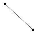 | |
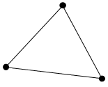
| Shell3 | CTRIA | 63,181 |
 | |
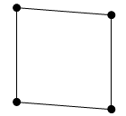
| Shell4 | CQUAD |
 | ||
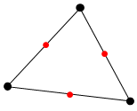
| Shell6 | CTRIA6 | 93, 281 |
 | |
| Shell8 | CQUAD8 |
 | ||
| Solid4 | CTETRA | 45,185 |
 | |
| Solid5 | CPYRA |
 | ||
| Solid6 | CPENTA |
 | ||
| Solid8 | CHEXA |
 | ||
| Solid10 | CTETRA | 92,95,186,187 |
 | |
| Solid13 | CPYRA |
 | ||
| Solid15 | CPENTA |
 | ||
| Solid20 | CHEXA |
 | ||
| FMASS | CONM2 | 21 | ||
| RBE2 (Rigid) | RBE2 | Rigid CERIG |
 | |
| RBE3 (Deformable) | RBE3 | Deformable RBE3 |
| |
The Motion solver provides an option that ensures the solution for solid elements is identical to the results obtained using the Mechanical APDL (MAPDL) solver. When this option is enabled, it matches the default settings of the MAPDL solver in analyses such as Static Structure or Transient Structure by utilizing the same shape functions and locations of integration points. This option is applicable to solid elements composed of isotropic and orthotropic materials.
The force and torque on the node are assembled from the elementary forces as follows.
 | (7–1) |
where:
 = elastic force by the element applied on the node = elastic force by the element applied on the node |
 = elastic torque by the element applied on the node = elastic torque by the element applied on the node |
 = element stiffness = element stiffness |
 = stiffness proportional damping (beta damping) = stiffness proportional damping (beta damping) |
 = step size scale factor for the damping matrix for beam and
shell elements = step size scale factor for the damping matrix for beam and
shell elements |
 = deformation of the node = deformation of the node |
 = time derivative of the deformation of the node = time derivative of the deformation of the node |
 = total number of elements in the nodal FE body = total number of elements in the nodal FE body |
βh is used to set the variable dependent on the step size for the damping matrix for beam and shell elements. The value of βh is as follows depending on the conditions.
 | (7–2) |
where:
 = step size = step size |
 = pre-defined factor. This value is preset to 0.01. = pre-defined factor. This value is preset to 0.01. |
Since this option is only available for beam and shell elements, the variable for solid elements (and EasyFlex elements) is always set to one.
For the general case, the element stiffness matrix is:
 | (7–3) |
where:
| B = partial derivative of the shape function for the finite element |
| D = strain-stress relationship matrix which is defined from the material properties. For more on D, see the Materials chapter. |
The nodal strain and stress are:
 | (7–4) |
 | (7–5) |
where:
| d = nodal displacement |
The Motion solver makes use of both standard and nonstandard numerical integration formulas. This section describes the numerical integration formulas used in the Motion solver.
Figure 7.2: Gauss Numerical Integration Constants
| No. Integration Points | Integration Point Locations (xi) | Weighting Factors (Hi) |
| 1 |
|
|
| 2 |
|
|
| 3 |
|
|
|
|
|


The integration points used for these triangles are given in the table below. L varies from 0.0 at an edge to 1.0 at the opposite vertex.
Figure 7.3: Numerical Integration for Triangles
| Type | Integration Point Locations | Weighting Factors |
| 1 Point Rule for Shell3 |
|
|
| 3 Point Rule for Shell6 |
|
|
|
|
| |
|
|
|


Element Type Employed: Shell3 (1 Point), Shell6 (3 Point)

The numerical integration of 2D quadrilaterals gives:
 | (7–6) |
where:
| f = function to be integrated |
| H = weighting factor |
| xi and yi = locations to evaluate function |
| l and m = number of integration (Gauss) points |
The integration point locations are shown in Figure 7.5: Integration Point Locations for Quadrilaterals. The locations and weighting factors can be calculated using Figure 7.2: Gauss Numerical Integration Constants twice.
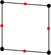
Element Type Employed: Shell4 (2x2), Shell8 (3x3)

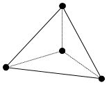
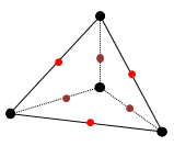
The integration points used for tetrahedra are given in the table below:
Figure 7.6: Numerical Integration for Tetrahedra
| Type | Integration Point Locations | Weighting Factors |
| 1 Point Rule for Solid4 |
|
|
| 3 Point Rule for Solid10 |
|
|
|
|
| |
|
|
| |
|
|
|


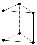
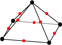
When the Element Consistency option is not enabled in the analysis settings, the integration points used for a pyramid is given in the table below.
Figure 7.8: Numerical Integration for Pyramids
| Type | Integration Point Locations | Weighting Factors | |
| 5 Point Rule for Solid5 |
Base Points |
|
|
|
|
| ||
|
|
| ||
|
|
| ||
|
Apex Point |
|
| |
| 9 Point Rule for Solid13 |
Base Points |
|
|
|
|
| ||
|
|
| ||
|
|
| ||
| Apex Point |
|
| |
| Edge Center Points |
|
| |
|
|
| ||
|
|
| ||
|
|
|


For 5-node pyramid element, when the Element Consistency option is enabled in the analysis settings, the 3D integration points(2x2x2) for 8-node solid elements are used in Equation 4.7. Here, it is assumed that nodes 5,6, 7 and 8 are located at the same position.
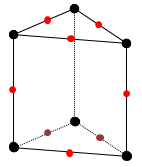
When the Element Consistency option is not enabled in the analysis settings, these wedge elements use an integration scheme that combines linear and triangular integrations, as shown in Figure 7.10: Integration Point Locations for Wedges. The locations and weighting factors can be calculated using Figure 7.2: Gauss Numerical Integration Constants and Figure 7.3: Numerical Integration for Triangles.

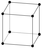
For 6-node wedge element, when the Element Consistency option is enabled in the analysis settings, the 3D integration points(2x2x2) for 8-node solid elements are used in Equation 7–7. Here, it is assumed that nodes 3 and 4, as well as nodes 7 and 8, are located at the same position.
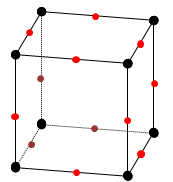
The 3D integration gives:
 | (7–7) |
and the integration point locations are shown in Figure 7.11: Integration Point Locations for Bricks. The locations and weighting factors can be calculated using Figure 7.2: Gauss Numerical Integration Constants three times.

In Finite Element Analysis, the evaluation of stress and strain at Gauss points provides a foundation for accurate internal state estimation within elements. Although direct evaluation at Gauss points produces precise data due to optimal integration accuracy, practical applications such as evaluating physical quantities on the structural surface necessitate the assessment of these quantities at the nodes.
The process to determine nodal stress and strain from Gauss point values involves extrapolation. This method uses the values computed at Gauss points located within the element to estimate values at the nodes. For an element with known stress or strain at its Gauss points, the extrapolation to the nodal points follows the approach outlined below:
Stress Evaluation at Gauss Points: Stress or strain is first calculated at the Gauss points based on the numerical integration of the governing equations. Once the nodal displacement is determined, strain and stress at Gauss element points can be calculated using Equation 7–4 and Equation 7–5.
Using Shape Functions for Extrapolation: The shape functions of each element are used to interpolate or extrapolate these values to the element nodes. For instance, in a 4-node quadrilateral element, the nodal stress can be extrapolated and estimated through the following process: A Gauss element is assumed based on the Gauss points.
The relationship between the natural coordinate system of the Gaussian element base and the natural coordinate system of the structural element base can be expressed proportionally as follows:

(7–8)
since
 ,
,  ,
,(7–9)
where:
rG = natural coordinate at gauss points with respect to the Gauss element rN = natural coordinate at gauss points with respect to the structure element r′G = natural coordinate at nodal points with respect to the Gauss element r′N = natural coordinate at nodal points with respect to the structure element Figure 7.13: Natural Coordinates of 4-Node Quadrilateral Element
Classification Index r s r′ s′ Structure Node 


Gauss Point 


Transformation from Gauss Points to Nodal Points for an Arbitrary Quantity u:

(7–10)
where:
Ni = ith shape functions of the element uN = quantity at the nodal point uG = quantity at the Gauss point This process ensures that the high precision obtained at the Gauss points due to numerical integration is effectively transferred to the more accessible nodal points for practical applications in engineering and analysis.
For linear, hyperelastic, and foam materials, extrapolated strain and stress values are reported. For plasticity materials, the method of reporting is dictated by the Plastic Strain option. For further information, See Strain-Stress Report for Plasticity Materials.

Note: For the nodal FE body, extrapolation is performed for all elements except for the constant strain Shell 3 and Solid 4 elements. For the modal FE body, strain and stress are derived from nodal displacements using the Motion Postprocessor. Extrapolation is performed exclusively for Shell 4, 6, 8, and Solid 8 elements.
A beam element is a basic element used to model elongated structural members subjected to various loading conditions. The stiffness and dynamic response of a beam element is mainly determined by its cross-sectional shape, which fundamentally influences its ability to resist bending, torsion, shear and axial loads. Beam elements are used in a wide variety of applications, from simple beams to more complex assemblies such as drive shafts, cables, automotive chassis, bridge structures, and mechanical frames.
The cross-sectional shape of a beam is a critical factor that determines its characteristics such as bending and torsion. Parameters dependent on the cross-sectional geometry, such as Cross-Sectional Area, Area Moment of Inertia, and Shear Area Ratio, define the properties of the beam. While these parameters can be user-defined, selecting a predefined Beam Cross Section Type and entering the geometric information allows for these parameters to be automatically calculated. Ansys Motion supports eight types of cross sections: Circular, Thin Tube, Hollow Circular, Elliptical, Rectangular, Hollow Rectangular, I-Beam, and T-Beam. Thin Tube and Elliptical types are supported only by Beam Group.
Note: In the Motion Standalone preprocessor, the PBeam property for NASTRAN requires users to manually input each parameter. For NASTRAN's PBeamL property, users can either select a predefined beam section and enter the geometric information or enter the parameters manually. The beam properties dependent on the geometry are calculated in the preprocessor, and the computed parameters are written to the solver input file(dfs).
The characteristics of a beam are defined by the parameters below.
| m = mass of the beam element |
| ρ = density |
| v = Poisson's ratio |
| E = Young's modulus |
| G = shear modulus |
| L = length of the beam element |
| A = area of cross section |
| Ixx = torsional constant |
| Iyy, and Izz = area moments of inertia about y, and z axis, respectively |
| Jxx, Jyy, and Jzz = mass moments of inertia about x, y, and z axis, respectively |
| Asy and Asz = shear area ratio about y, and z axis, respectively |
The mass and the moment of inertia about the x-axis of a nodal body for a beam element are calculated using the equations below:
 | (7–11) |
 | (7–12) |
The torsional constant of a beam element can be calculated using the equation below:
 | (7–13) |
Note: If the specified y-axis is defined to be parallel to the relative displacement between the two markers for the beam element, an error will be returned.
A circular cross section is defined as follows:

where:
| R = radius of the circle, and R>0. |
Beam and material properties for a circular cross section are defined as:
 | (7–14) |
 | (7–15) |
 | (7–16) |
 | (7–17) |
A thin tube cross section is defined as follows:

where:
| R = radius of the circle, and R>0 |
| t = thickness of the tube |
Beam and material properties for a thin tube cross section are defined as:
 | (7–18) |
 | (7–19) |
 | (7–20) |
 | (7–21) |
A hollow circular cross section is defined as follows:

where:
| Ro = outer radius of the circle, and Ro>0. |
| Ri = inner radius of the circle. Ri>0 and Ri<Ro . |
Beam and material properties for a hollow circular cross section are defined as:
 | (7–22) |
 | (7–23) |
 | (7–24) |
 | (7–25) |
where:
 | (7–26) |
An elliptical cross section is defined as follows:

where:
| a = semi length of the z-axis of the ellipsoid |
| b = semi length of the y-axis of the ellipsoid |
Beam and material properties for an elliptical cross section are defined as:
 | (7–27) |
 | (7–28) |
 | (7–29) |
 | (7–30) |
 | (7–31) |
 | (7–32) |
 | (7–33) |
A rectangular cross section is defined as follows:

where:
| h = length of the y-axis of the box |
| b = length of the z-axis of the box |
Beam and material properties for a rectangular cross section are defined as:
 | (7–34) |
 | (7–35) |
 | (7–36) |
 | (7–37) |
 | (7–38) |
 | (7–39) |
A hollow rectangular cross section is defined as follows:

where:
| h = length of hollow rectangular in y-axis direction |
| b = length of hollow rectangular in z-axis direction |
| ty = thickness of hollow rectangular in y-axis direction |
| tz = thickness of hollow rectangular in z-axis direction |
Beam and material properties for a hollow rectangular cross section are defined as:
 | (7–40) |
 | (7–41) |
 | (7–42) |
 | (7–43) |
 | (7–44) |
 | (7–45) |
 | (7–46) |
where:
 | (7–47) |
An i-beam cross section is defined as follows:

where:
| h = web length of the y-axis of the I-beam |
| b = length of the z-axis of the I-beam |
| tw = web thickness of the z-axis of the I-beam |
| tf = flange thickness of the y-axis of the I-beam |
Beam and material properties for an i-beam cross section are defined as:
 | (7–48) |
 | (7–49) |
 | (7–50) |
 | (7–51) |
 | (7–52) |
 | (7–53) |
 | (7–54) |
where:
 | (7–55) |
 | (7–56) |
A t-beam cross section is defined as follows:

where:
| h = length of the y-axis of the T-beam |
| b = length of the z-axis of the T-beam |
| tw = web thickness of the z-axis of the T-beam |
| tf = flange thickness of the y-axis of the T-beam |
Beam and material properties for a t-beam cross section are defined as:
 | (7–57) |
 | (7–58) |
 | (7–59) |
 | (7–60) |
 | (7–61) |
 | (7–62) |
 | (7–63) |
where:
 | (7–64) |
 | (7–65) |
 | (7–66) |
A 2-Node beam element is a linear element where one element is defined from two 6-DOFs nodes.

Element Reference Frame
Beam properties such as area moment of inertia must be defined in the beam reference frame.

The x-axis of the beam reference frame can be determined from the relative displacement between two nodes as follows.
 | (7–67) |
The y and z-axes of the beam reference frame are determined from the user-defined direction vector and x-axis as follows.
 | (7–68) |
 | (7–69) |
Therefore,
 | (7–70) |
where:
| r1 and r2 = position vectors of two nodes |
| yuser = user-defined direction vector |
| x, y and z = x, y, and z axes of the beam reference frame, respectively |
| Ae = element reference frame |
Shape Functions
 | (7–71) |
 | (7–72) |
 | (7–73) |
 | (7–74) |
 | (7–75) |
 | (7–76) |
 | (7–77) |
 | (7–78) |
 | (7–79) |
 | (7–80) |
 | (7–81) |
 | (7–82) |
 | (7–83) |
 | (7–84) |
with
 | (7–85) |
 | (7–86) |
Here, θmn is the rotations about the local m-axis at node n.
Shell elements are used to model thin structures, such as plates and films. They require less computational effort than solid elements, while still providing detailed and accurate predictions of stress, strain, and deformation in curved shell structures. Shell elements are utilized across a wide range of applications, from simple structures like wall panels and speaker plates to complex curved surfaces found in battery films, automotive chassis, and aircraft fuselages.

3-Node Triangular is a linear shell element where an element is defined by three 6-DOFs nodes.
Shape Functions
 | (7–87) |
 | (7–88) |
 | (7–89) |
 | (7–90) |
 | (7–91) |
 | (7–92) |
 | (7–93) |
 | (7–94) |
 | (7–95) |
Here, θmn is the rotation about the local m-axis at node n.
4-Node Quadrilateral is a linear shell element where an element is defined by four 6-DOFs nodes.
Shape Functions
 | (7–96) |
 | (7–97) |
 | (7–98) |
 | (7–99) |
 | (7–100) |
 | (7–101) |
 | (7–102) |
 | (7–103) |
 | (7–104) |
 | (7–105) |
Here, θmn is the rotation about the local m-axis at node n.
6-Node Triangular is a linear shell element where an element is defined by six 6-DOFs nodes.
Shape Functions
 | (7–106) |
 | (7–107) |
 | (7–108) |
 | (7–109) |
 | (7–110) |
 | (7–111) |
 | (7–112) |
 | (7–113) |
 | (7–114) |
 | (7–115) |
 | (7–116) |
 | (7–117) |
Here, θmn is the rotation about the local m-axis at node n.


Solid elements are employed to model three-dimensional structures with complex geometries that exhibit substantial depth, width, and height. These elements are crucial in finite element analysis (FEA) for representing various shapes, ranging from simple rectangular blocks to the complex and irregular forms commonly found in automotive components and industrial machinery. Solid elements are particularly valuable for their ability to analyze multi-axial stress and strain, providing essential data for evaluating the structural integrity and mechanical performance of components under real-world conditions. Their application is comprehensive in calculating stress-strain relationships, making precise modeling indispensable in engineering domains such as automotive design and aerospace, where safety and functionality are impacted.
4-Node Tetrahedra are linear solid elements where an element is defined by four 3-DOFs nodes.

Shape Functions
 | (7–132) |
 | (7–133) |
 | (7–134) |
 | (7–135) |
 | (7–136) |
 | (7–137) |
 | (7–138) |
5-Node Pyramids are linear solid elements where an element is defined by five 3-DOFs nodes.

Shape Functions
 | (7–139) |
 | (7–140) |
 | (7–141) |
 | (7–142) |
 | (7–143) |
 | (7–144) |
 | (7–145) |
 | (7–146) |
6-Node Wedges are linear solid elements where an element is defined by six 3-DOFs nodes.

Shape Functions
 | (7–147) |
 | (7–148) |
 | (7–149) |
 | (7–150) |
 | (7–151) |
 | (7–152) |
 | (7–153) |
 | (7–154) |
 | (7–155) |
8-Node Bricks without ESF (Extra Shape Function) are used for solid8 elements when the Element Consistency option is not enabled. This element is defined by eight 3-DOFs nodes.

Shape Functions
These shape functions are for 8-node brick elements without extra shape functions.
 | (7–156) |
 | (7–157) |
 | (7–158) |
 | (7–159) |
 | (7–160) |
 | (7–161) |
 | (7–162) |
 | (7–163) |
 | (7–164) |
 | (7–165) |
 | (7–166) |
8-Node Bricks with ESF (Extra Shape Function) are used for solid8 elements when the Element Consistency option is enabled. This element is defined by eight 3-DOFs nodes and three extra 3-DOFs nodes.
Shape Functions
These shape functions are for 8-node brick elements with extra shape functions.
 | (7–167) |
 | (7–168) |
 | (7–169) |
 | (7–170) |
 | (7–171) |
 | (7–172) |
 | (7–173) |
 | (7–174) |
 | (7–175) |
 | (7–176) |
 | (7–177) |
 | (7–178) |
 | (7–179) |
 | (7–180) |
10-Node Tetrahedra are high-order solid elements where an element is defined by ten 3-DOFs nodes.

Shape Functions
 | (7–181) |
 | (7–182) |
 | (7–183) |
 | (7–184) |
 | (7–185) |
 | (7–186) |
 | (7–187) |
 | (7–188) |
 | (7–189) |
 | (7–190) |
 | (7–191) |
 | (7–192) |
 | (7–193) |
13-Node Pyramids are high-order solid elements where an element is defined by thirteen 3-DOFs nodes.

Shape Functions
 | (7–194) |
 | (7–195) |
 | (7–196) |
When the Element Consistency option is not enabled in the analysis settings:
 | (7–197) |
 | (7–198) |
 | (7–199) |
 | (7–200) |
 | (7–201) |
 | (7–202) |
 | (7–203) |
 | (7–204) |
 | (7–205) |
 | (7–206) |
 | (7–207) |
 | (7–208) |
 | (7–209) |
When the Element Consistency option is enabled in the analysis settings:
 | (7–210) |
 | (7–211) |
 | (7–212) |
 | (7–213) |
 | (7–214) |
 | (7–215) |
 | (7–216) |
 | (7–217) |
 | (7–218) |
 | (7–219) |
 | (7–220) |
 | (7–221) |
 | (7–222) |
15-Node Wedges are high-order solid elements where an element is defined by fifteen 3-DOFs nodes.

Shape Functions
 | (7–223) |
 | (7–224) |
 | (7–225) |
 | (7–226) |
 | (7–227) |
 | (7–228) |
 | (7–229) |
 | (7–230) |
 | (7–231) |
 | (7–232) |
 | (7–233) |
 | (7–234) |
 | (7–235) |
 | (7–236) |
 | (7–237) |
 | (7–238) |
 | (7–239) |
 | (7–240) |
20-Node Bricks are high-order solid elements where an element is defined by twenty 3-DOFs nodes.

Shape Functions
 | (7–241) |
 | (7–242) |
 | (7–243) |
 | (7–244) |
 | (7–245) |
 | (7–246) |
 | (7–247) |
 | (7–248) |
 | (7–249) |
 | (7–250) |
 | (7–251) |
 | (7–252) |
 | (7–253) |
 | (7–254) |
 | (7–255) |
When the Element Consistency option is not enabled in the analysis settings:
 | (7–256) |
 | (7–257) |
 | (7–258) |
 | (7–259) |
 | (7–260) |
 | (7–261) |
 | (7–262) |
 | (7–263) |
When the Element Consistency option is enabled in the analysis settings:
 | (7–264) |
 | (7–265) |
 | (7–266) |
 | (7–267) |
 | (7–268) |
 | (7–269) |
 | (7–270) |
 | (7–271) |