


This section introduces the generalized coordinate and coordinate system used by the Motion application. It lays the groundwork for understanding how the Motion solver models and analyzes the movement of bodies within a multibody system. By defining bodies in terms of their positions and orientations relative to a coordinate system, you can accurately simulate the dynamics of complex systems. This section explores the essential components that make up the kinematics of multibody systems, including how bodies are defined, how their movement is represented, and how these representations are crucial for detailed analysis. This foundation is critical for anyone looking to explore the intricate behaviors of interconnected bodies in motion.
A generalized coordinate denotes a variable specifying either position or orientation measured from a coordinate system. Consider a particle in a plane. This particle can be located by r and θ in the polar coordinate system. The same particle also can be located by x and y coordinates in the Cartesian coordinate system. We refer to r and θ, as well as x and y, as generalized coordinates.

It is very important to know that all governing equations must be expressed in terms of generalized coordinates and their derivatives. Generalized coordinates are therefore unknowns to be found from the governing equations.
Note: The Motion solver utilizes a total of six Cartesian generalized coordinates to represent the three translational and three rotational motions of a body in three-dimensional space.
Coordinate systems are one of the essential elements used to express the position and orientation of any object used in Motion. A coordinate system is defined to measure physical quantities. Any physical quantity must be measured from the coordinate system. It is used to measure the position and orientation of a body, relative displacements and angles, and their time derivatives, between bodies (nodes) to which they belong.
A marker is a specialized coordinate system defined on a body or node, enabling result reporting and referencing by other entities. By defining a coordinate system with a marker, results such as the marker's position, velocity, and acceleration can be tracked in the postprocessor. Additionally, markers can be referenced in function expressions, user subroutines, and other Motion entities. Markers are automatically created at the center of mass of a rigid body, at joints, and at some force entities. You can also create markers at desired locations to define custom coordinate systems.
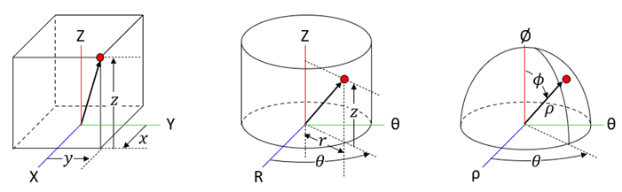
Motion accommodates the Cartesian, Cylindrical, and Spherical types of coordinate system, with the Motion solver exclusively utilizing the Cartesian type. The remaining two types, Cylindrical and Spherical, find their application in the preprocessing and postprocessing stages.
- Cartesian Coordinate Systems
This system facilitates the representation of a vector through its x, y, and z components within the Cartesian framework.
- Cylindrical Coordinate Systems
In this system, a vector is articulated via its r, θ, and z components, adhering to the cylindrical coordinate methodology.
- Spherical Coordinate Systems
This approach allows for the expression of a vector through its ρ, θ, and φ components, conforming to the spherical coordinate convention.
- Global Coordinate System
The Global Coordinate System is a stationary reference frame within a simulation or modeling environment, providing a uniform basis for defining positions, orientations, and movements across all model elements. This system is fixed, organized as a Cartesian coordinate grid with x, y, and z axes originating from (0,0,0). In Motion, it is also referred to as the Inertial Reference Frame.
- Local (Body) Coordinate System
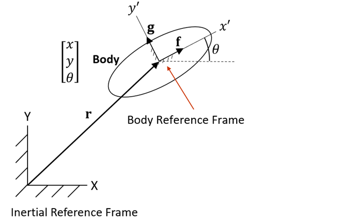
Attached to individual bodies, these coordinate systems move and rotate with the body. The Body Reference Frame is a type of this coordinate system. Additionally, a local coordinate system is created when markers or joints are created on a body or node in the preprocessor.
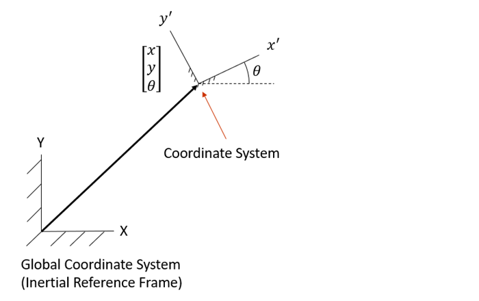
To define a coordinate system in a plane, position vector and orientation matrices are used to express its location. In 2-dimensional space, a vector made up with three scalar values (x,y,θ) can simply be used.
To define the position and orientation of a body within a system, a Body Reference Frame is employed. This system of coordinates, which includes generalized coordinates, specifies the body's position and orientation relative to the inertial reference frame.
The position of the body reference frame in a plane is defined from the position
vector  .
.
 | (2–1) |
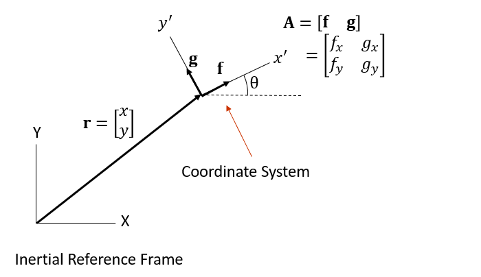
The x' and y' axes of the body reference frame are defined from the unit vectors f and g perpendicular to each other, respectively.
 | (2–2) |
 | (2–3) |
Here, cosθ and sinθ are the direction cosines that facilitate the rotational transformation from the body reference frame to the inertial reference frame.
The transformation matrix, denoted as A, encapsulates the orientation of a coordinate system in the plane and is defined as:
(2–4) |
Where, f and g are direction cosines of the coordinate system.
A transformation matrix is also called an orientation matrix because it represents the orientation of the coordinate system, and a rotation matrix because it represents the rotation of the coordinate system. A transformation matrix allows for the conversion of vectors from the body reference frame to the inertial reference frame and vice versa.
The inverse of the transformation matrix A is simply transpose of matrix A:
(2–5) |
Thus:
 | (2–6) |
This demonstrates that A is orthogonal. Such a property simplifies switching between local and global coordinate systems, making transformations easier for accurate modeling and analysis in multibody dynamics.
This section describes coordinate system transformations between coordinate systems or between coordinate system types.
It is often necessary to express a vector in many different coordinate systems. In order to express a vector in two different coordinate systems, we need to carry out the coordinate transformation. The coordinate transformation matrix can be developed by geometric relationship as in the figure below.
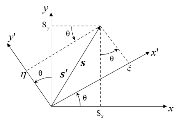
Whenever a vector is multiplied by a coordinate transformation matrix, the resulting vector is the same vector expressed in other coordinate system. The equations below examine the two vectors s and s′ from the figure above.
 | (2–7) |
 | (2–8) |
There exists the following relationship between two vectors. This relationship can be easily derived from the basics of geometry.
 | (2–9) |
Hence, to represent a vector s′ from its local coordinate system to the inertial reference frame:
 | (2–10) |
For the reverse process, transform a vector from the inertial reference frame to the local coordinate system:
 | (2–11) |

