


Building on the two-dimensional analysis foundation, this section examines defining, positioning, and orienting bodies in three-dimensional space. This is a crucial step for precise dynamics analysis in Motion. Our focus is to equip readers with the skills to navigate Motion's three-dimensional capabilities, enhancing both simulation accuracy and our understanding of mechanical behaviors.
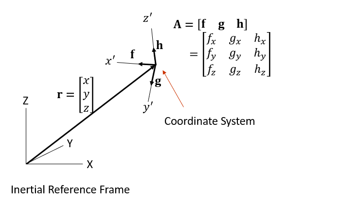
To define the position and orientation of the coordinate system in three-dimensional space, we start with the position of the body reference frame, which is determined by the position vector r.
 | (2–18) |
Following this, the coordinate system's x′, y′, and z′ axes can be defined from the unit vectors f, g, and h that are perpendicular to each other, respectively. These vectors not only define the orientation of the body in space but also form the columns of the orientation matrix A, which is used to transform coordinates from the body reference frame to the inertial reference frame.
 | (2–19) |
Euler angles represent a classical set of orientation parameters used to describe the orientation of coordinate systems in three-dimensional space. This method employs three sequential rotations about the axes of a coordinate system. The concept extends from a simpler process, where a single rotation angle specifies orientation in a plane, to a more complex one that can capture orientation in three dimensions.
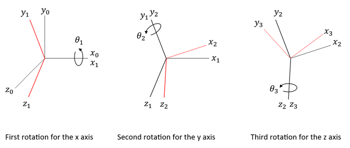
This section introduces the XYZ Euler angle convention, a method for defining the orientation of coordinate systems through sequential rotations around the X, Y′, and Z″ axes, denoted by angles θ1, θ2 and θ3, respectively. Selected for its clarity, the XYZ convention exemplifies the core concepts of Euler angles, facilitating the understanding and application of various conventions in multibody dynamics analyses.
First Rotation (θ1 about x-axis)
The first rotation by an angle θ1 occurs about the original x-axis of the fixed coordinate system. This rotation tilts the coordinate system, altering its orientation by pivoting around the x-axis without affecting the position of the axis itself. The transformation matrix for this rotation, denoted as Rx (θ1), incorporates cosθ1 and sinθ1 to adjust the y and z-coordinates accordingly, while the x-coordinates remain unchanged.
 | (2–20) |
Second Rotation (θ2 about y-axis)
Following the first rotation, the second rotation by angle θ2 is executed around the y-axis. At this point, the y-axis itself remains fixed in space, but the orientation of the coordinate system changes by pivoting around this axis. The rotation affects the x and z-coordinates, represented in the transformation matrix Ry(θ2) which includes terms involving cosθ2 and sinθ2, indicating the rotation's impact on these axes.
| (2–21) |
Third Rotation (θ3 about z-axis)
The final rotation by an angle θ3 takes place around the x-axis. This rotation completes the sequence, bringing the body to its desired orientation. The transformation matrix Rz(θ3) uses cosθ3 and sinθ3 to modify the x and y-coordinates, reflecting the body's rotation around the z-axis.
 | (2–22) |
Combined Transformation
The overall orientation of the coordinate system in the fixed coordinate system is achieved by sequentially applying these three rotations. The combined effect is represented by the product of the individual orientation matrices:
(2–23) |
This is the general form of an orientation matrix for representing the orientation of a coordinate system in three-dimensional space.
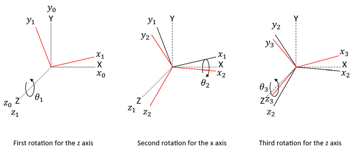
For the ZYX Euler angle sequence, the orientation is defined by three sequential rotations around the Z, Y′, and X″ axes, denoted by angles θ1(psi), θ3(theta) and θ3(phi). This approach is another classical method used to define the orientation of coordinate systems in 3D. Similar to the XYZ Euler angle, the overall orientation of the coordinate system relative to the fixed coordinate system is achieved after the three rotations are applied sequentially. The combined transformation matrix for the ZYX Euler angles is calculated as the product of the individual rotation matrices:
 | (2–24) |
For the ZXZ Euler angle sequence, the orientation is defined by three sequential rotations about the Z, X′, and Z″ axes, denoted by angles θ1(yaw), θ3(pitch) and θ3(roll). Similar to the XYZ Euler angle, the overall orientation of the coordinate system relative to the fixed coordinate system is achieved after the three rotations are applied sequentially. The combined transformation matrix for the ZXZ Euler angles is calculated as the product of the individual rotation matrices:
 | (2–25) |
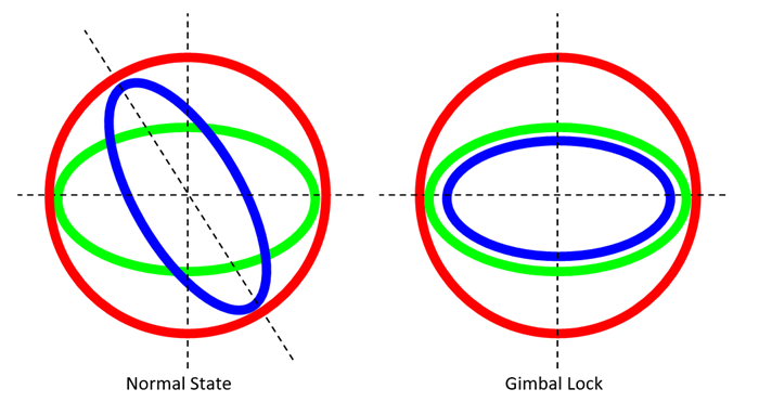
When discussing Euler angles in multi-body dynamics, the phenomenon of singularity is an important factor to consider. Singularity occurs when two rotation axes align due to the chosen sequence of rotations in a specific direction. This alignment is known as gimbal lock, and it results in the loss of one degree of rotational freedom. In fact, the system enters a state where it cannot uniquely determine the orientation of the body because the two axes overlap. This situation not only complicates the process of calculating direction but also poses a significant challenge in accurately simulating and analyzing the dynamics of the system.
One effective strategy to circumvent the issue of singularity is to switch between different Euler angle conventions as the system approaches a known singularity. For instance, if the simulation or analysis in the XYZ convention is nearing a configuration that would result in gimbal lock (where rotational axes align and cause a loss of a degree of freedom), transitioning to the ZYX convention might offer a set of rotations that does not suffer from the same singular configuration. Similarly, switching to the ZXZ or ZXY conventions can provide alternative sequences of rotations that mitigate the risk of encountering a singular orientation.
By monitoring the angles of rotation, especially the second rotation in the sequence which typically leads to gimbal lock if it approaches 0 or 180 degrees, the system can automatically switch to an alternative Euler angle convention before the singularity is reached.
The Motion solver intelligently selects the most appropriate Euler angle convention from various options to avoid potential singularities. By proactively identifying orientations that could lead to gimbal lock, it dynamically switches among conventions such as ZYX, ZXZ, and ZXY. This adaptability allows for the preservation of simulation integrity across diverse orientations, ensuring that the intrinsic constraints of Euler angles do not compromise the analysis of intricate dynamic systems.
Fixed angles are a set of three angles that describe the orientation of a coordinate system or body in a three-dimensional space by performing sequential rotations around fixed axes. Unlike Euler angles, which define the orientation by rotations about axes that may change their orientation after each rotation, fixed angles involve rotations about axes that remain static relative to the specific coordinate frame from the start to the end of the sequence. Fixed angles can often provide a more intuitive understanding of the rotation of a coordinate system due to their consistent reference frame throughout the rotation process.
For instance, in the case of ZXZ Euler angles, the orientation is defined through rotations about the Z, X′, and Z″ axes, and the orientation matrix is calculated as in Equation 2–25. Conversely, fixed angles perform the rotations in the reverse order compared to Euler angles. The sequence for fixed angles would therefore be around the Z, X, and Z axes, and the corresponding orientation matrix is:
 | (2–26) |
This reversal in the order of rotations is the primary distinction in how fixed angles are conceptualized compared to Euler angles.
Note that fixed angles are not used in the Motion solver, but are used when defining the orientation of a body or coordinate system in the Motion standalone preprocessor. Here, the fixed reference coordinate system for calculating the fixed angles is the inertial reference frame.
The position rp and orientation Ap of the coordinate system, defined at an arbitrary point P on the ith body, can be written as:
 | (2–27) |
 | (2–28) |
where
| ri = position of the ith body reference frame |
| Ai = orientation of the ith body reference frame |
| si = relative position vector with respect to the inertial reference frame |
| s′i = relative position vector with respect to the body reference frame |
| Ci = relative orientation matrix. This is the orientation of the local reference frame with respect to the body reference frame. |
| rp = position of the coordinate system on a ith rigid body |
| Ap = orientation of the coordinate system on a ith rigid body |
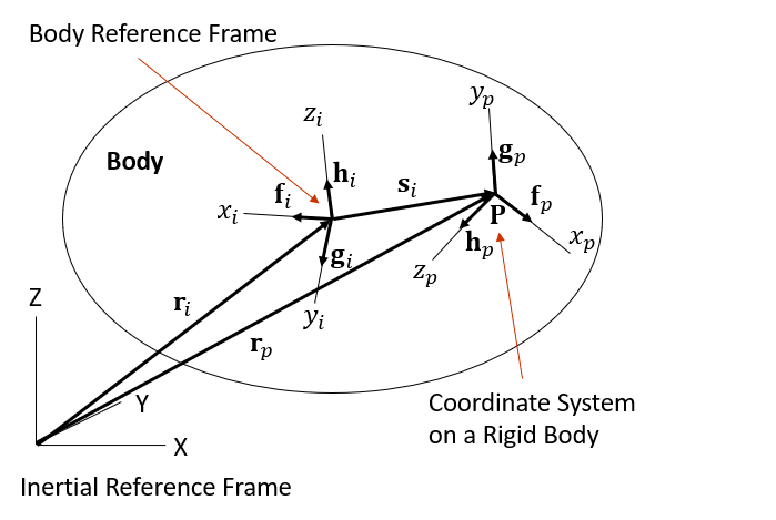
The orientation of Ap can be described either through Euler Angles or by using the direction vectors fp, gp and hp, which align with the axes of the coordinate system.
If the body is a rigid body type and not permit deformation, the coordinate system defined at point P moves and rotates with the rigid body, while s′i and Ci remain constant and are calculated as follows:
 | (2–29) |
 | (2–30) |
The translational velocity of a body reference frame with respect to the inertial reference frame can be written as:
 | (2–31) |
The angular velocity with respect to the inertial reference frame is:
 | (2–32) |
For the XYZ Euler Angle, w′i can be expressed from the Euler angles and their time derivatives.
 | (2–33) |
where:
DXYZ = angular velocity transformation matrix for the XYZ Euler angle and is:
 | (2–34) |
 | (2–35) |
The angular velocity with respect to the inertial reference frame is:
 | (2–36) |
The translational velocity of the coordinate system on a body with respect to the inertial reference frame can be derived as follows:
 | (2–37) |
where:
 | (2–38) |
where  and
and  are skew-symmetric matrix and can be
written as:
are skew-symmetric matrix and can be
written as:
 | (2–39) |
When there is no deformation in the body, the angular velocity is constant at all points on the body, the angular velocity of the coordinate system on a body with respect to the body reference frame is:
 | (2–40) |
The accelerations of the marker in the inertia reference frame can be defined as follows:
 | (2–41) |
The translational acceleration of a body reference frame with respect to the inertial reference frame can be written as:
 | (2–42) |
The angular acceleration is a vector measured with respect to its own body reference frame, and is therefore typically expressed in the local coordinate system.
 | (2–43) |
For the XYZ Euler Angle,  can be expressed from the Euler angles and their first and
second time derivatives.
can be expressed from the Euler angles and their first and
second time derivatives.
 | (2–44) |
where:
 | (2–45) |
 | (2–46) |
The translational acceleration of the coordinate system on a body with respect to the inertial reference frame is:
 | (2–47) |
When there is no deformation in the body, the angular acceleration is constant at all points on the body, the angular acceleration of the coordinate system on a body with respect to the body reference frame is:
 | (2–48) |