In multibody dynamics simulations, constraints are essential components that limit the movement of objects within a mechanical system. They are expressed as algebraic equations related to the system’s generalized coordinates. These equations define the permissible movements between joints and other bodies, ensuring that the objects move in accordance with the physical and mechanical laws imposed by the constraints. The constraint equations are nonlinear and must be continuously satisfied throughout the simulation process, ensuring that the movements of the objects comply with the limits and interactions directed by the physical setup of the system. Each joint within the system is typically defined by one or more of these constraint equations, specifying the relative movements allowed between the connected bodies.
This section explores the application and management of constraints in multibody dynamics, including the Lagrange Multiplier Method for strict enforcement of constraints and the Penalty Based Method for a softer, more stable approach. It also discusses the challenges and solutions related to Redundant Constraints and Singular Configurations, which can complicate simulations and affect system stability and accuracy.
There are two types of constraint equations: Kinematic and Driving constraints.
Kinematic Constraints
Kinematic constraints originate from the geometric conditions imposed by joints connecting bodies. They restrict relative motion to a predefined motion path. Typical examples include revolute, translational, and spherical joints, each allowing specific types of relative motion while constraining others. These are denoted by the superscript K as follows:
 | (2–125) |
Driving Constraints
Also known as motion constraints, driving constraints are imposed by forces or prescribed motions that influence the dynamic behavior of the system. These constraints often enforce specific motion trajectories or speed profiles over time. These are denoted by the superscript D as follows:
 | (2–126) |
Combined Constraints
Combining these two constraints gives the following constraint equations:
 | (2–127) |
Constraints in a multibody system must be comprehensively enforced at three primary levels: position, velocity, and acceleration.
Position Constraints: Position constraints dictate that the configuration of the system must comply with the geometric, joint, or driving constraints at the position level. These are usually expressed in the form of algebraic equations involving the generalized coordinates of the bodies.
Velocity Constraints: Velocity constraints are the time derivatives of the position constraints or driving constraints at the velocity level.
Acceleration Constraints: Acceleration constraints are the second time derivatives of the position constraints or driving constraints at the acceleration level.
During initial analyses such as position, velocity, and acceleration studies, appropriate constraint equations corresponding to each level must be satisfied. In static and eigenvalue analyses, only the position constraints are required to be met. Conversely, during dynamic analyses, it is imperative to satisfy constraints at all three levels: position, velocity, and acceleration.
Example of Position, Velocity and Acceleration Level Constraints
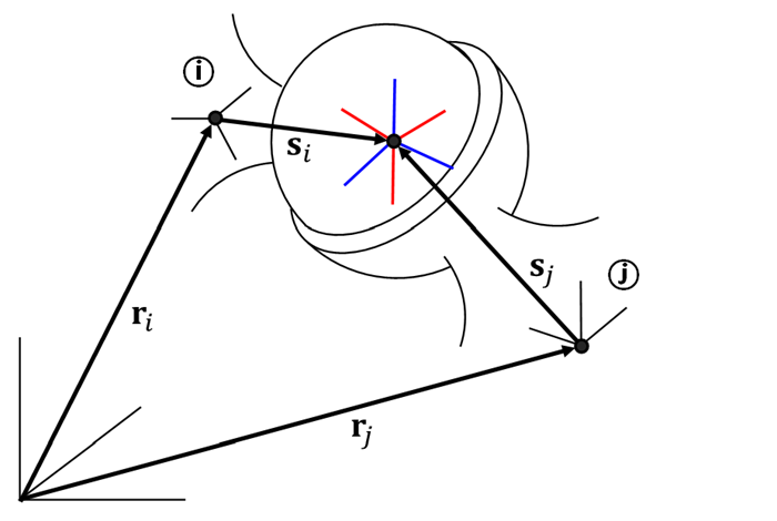
To illustrate how these constraints operate at different levels, consider a revolute joint connecting two bodies in a 2D plane:
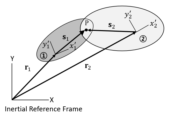
A revolute joint allows relative rotation about a point P common to bodies 1 and 2, as shown in the figure above. Since point P must coincide, the vector additions to locate point P must be equal. Therefore, the constraint equation at the position level is
 | (2–128) |
where:
 | (2–129) |
 | (2–130) |
 | (2–131) |
Taking the time derivative of the constraint yields the following velocity level constraint equation:
 | (2–132) |
where:
B = partial derivative of the orientation matrix A with respect to the angle θ and is:
 | (2–133) |
Equation 2.131 can be rewritten as:
 | (2–134) |
where:
 = constraint Jacobian matrix and is:
 | (2–135) |
 = time derivatives of generalized coordinates and is:
 | (2–136) |
Taking the second time derivatives of the constraint yields the following acceleration level constraint:
 | (2–137) |
where:
 = second time derivatives of generalized coordinates and
is:
= second time derivatives of generalized coordinates and
is:
 | (2–138) |
 = velocity term of the constraint equation at the acceleration
level and is:
= velocity term of the constraint equation at the acceleration
level and is:
 | (2–139) |
This section introduces the most fundamental constraints used in joint definitions. A joint is composed of a combination of these basic constraints. The following examples illustrate how typical joints can be formed by combining the basic constraints discussed in this section:
Revolute Joint: Two Dot1 Constraint + Spherical Constraint
Translational Joint: Three Dot1 Constraint + Two Dot2 Constraint
Fixed Joint: Three Dot1 Constraint + Spherical Constraint
Cylindrical Joint: Parallel Constraint + Two Dot2 Constraint • Ball Joint: Spherical Constraint
Universal Joint: Dot1 Constraint + Spherical Constraint
Planar Joint: Two Dot1 Constraint + Dot2 Constraint
Distance Joint: Distance Constraint
Parallel Joint: Parallel Constraint
Orientation Joint: Orientation Constraint
The combinations introduced above represent the basic concept of constructing joints using basic constraints. For the detailed formulation of each joint, refer to the specific sections for each type of joint in this guide.
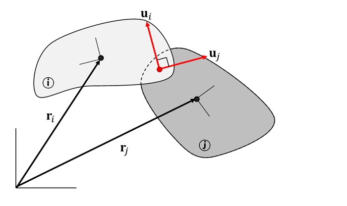
The Dot1 constraint is the most basic constraint indicating that two vectors are orthogonal. The Dot1 constraint equation is:
 | (2–140) |
where:
| ui and uj = nonzero vectors fixed to bodies i and j, respectively |
| Ai and Aj = orientation matrix of bodies i and j, respectively |
| u′i and u′j = vectors fixed to body i and j with respect to their own body, respectively |
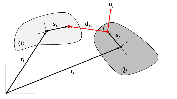
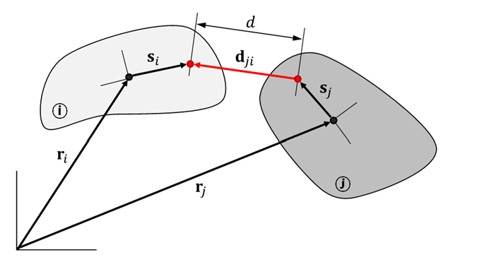
The Dot2 constraint defines the condition where a fixed vector on one body is orthogonal to a relative vector between arbitrary points on each body. The Dot2 constraint equation is:
 | (2–141) |
where:
| dji = relative position vector between two points on bodies i and j and is defined as: |
 | (2–142) |
The Spherical constraint allows two bodies to rotate freely about a point in three-dimensional space, defined by the condition that the coordinates of two coordinate systems, each fixed on a body, coincide. The spherical constraint equation is:
 | (2–143) |
The Distance constraint ensures that each point on two bodies maintains a constant distance. It functions like a rod with spherical joints at each point. The distance constraint equation is:
 | (2–144) |
where:
| d = constant distance that must be maintained between the two points on the respective bodies |
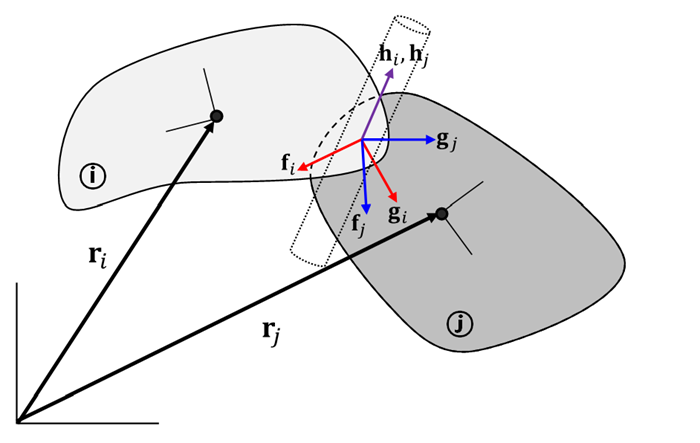
The Parallel constraint ensures that one axis of two coordinate systems, defined on each body, remains parallel. The parallel constraint equation that keeps the hi and hj, which correspond to the z-axes of each coordinate system is:
 | (2–145) |
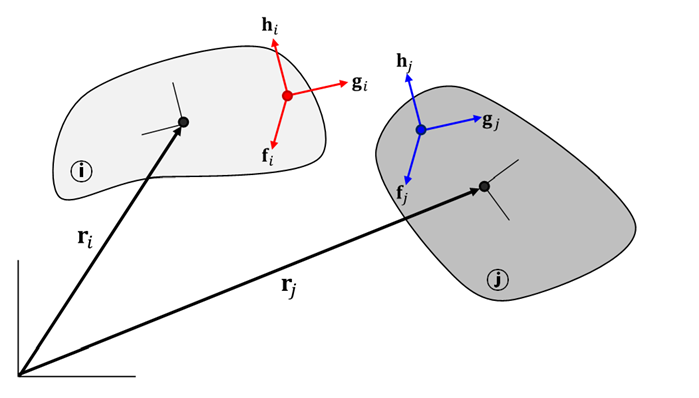
The Orientation constraint ensures that the orientations of two coordinate systems, defined on each body, are identical to each other. The orientation constraint equation is:
 | (2–146) |
A Rotational motion constraint is a type of driving constraint applied to the rotational degrees of freedom in dynamic systems. These constraints control the relative angular displacement, relative angular velocity, and relative angular acceleration of joints to follow a predetermined rotational trajectory, speed, or angular acceleration profile.
In a rotational system, the orientation of the action marker relative to the base marker can be calculated as:
 | (2–147) |
where:
| Aa = the orientation of the action marker |
| Ab = the orientation of the base marker |
If rotational motion is allowed only along the z-axis of the joint's coordinate system, Equation 2.146 can be rewritten as follows:
 | (2–148) |
where:
θba = relative angular displacement between two markers, calculated as:
 | (2–149) |
where:
N = the number of complete rotations
The relative angular velocity and acceleration can be represented as follows:
 | (2–150) |
 | (2–151) |
where:
 = the angular velocity of the action marker = the angular velocity of the action marker |
 = the angular velocity of the base marker = the angular velocity of the base marker |
 = the angular acceleration of the action marker = the angular acceleration of the action marker |
 = the angular acceleration of the base marker = the angular acceleration of the base marker |
 = z-axis vector in the base marker's orientation = z-axis vector in the base marker's orientation |
 = the first time derivative of z-axis vector in the
base marker's orientation = the first time derivative of z-axis vector in the
base marker's orientation |
The driving constraint equations in the position, velocity and acceleration levels can be defined using the rotational angle and its time derivatives of Equation 2–149 ∼ Equation 2–151 as follows:
 | (2–152) |
 | (2–153) |
 | (2–154) |
where:
F = a function defined by a Motion Function Expression or User Subroutine.
The function F can be dependent on the displacement, velocity, acceleration of other bodies, variable and differential equation, and time. The driving torque is defined from Lagrange multiplier and added to the constrained force from Equation 2.167 as follows:
 | (2–155) |
where:
 = driving torque = driving torque |
 = Lagrange multiplier for the rotational constraint
equations = Lagrange multiplier for the rotational constraint
equations |
 = Lagrange multiplier for the rotational motion
constraint = Lagrange multiplier for the rotational motion
constraint |
Note: Since, from Equation 2–147, this entity can cause a problem for a solution step when the rotating angle exceeds π in one time step, the Motion solver shows a warning message in the message file under dynamic analysis. The warning condition is when the rotation velocity * step size is bigger than π. In this case, you must set the maximum step size to a smaller value in order to avoid the problem. This situation only occurs when a body rotates at extreme speeds.
A Translational motion constraint is a type of driving constraint applied to the translational degrees of freedom in dynamic systems. These constraints control the relative translational displacement, relative translational velocity, and relative translational acceleration of joints to follow a predetermined translational trajectory, speed, or translational acceleration profile.
If translational motion is allowed only along the z-axis of the joint's coordinate system, the relative displacement, velocity and acceleration of the action marker relative to the base marker can be calculated as:
(2–156) |
(2–157) |
(2–158) |
where:
 = relative displacement in the z-direction between the
action and base markers = relative displacement in the z-direction between the
action and base markers |
 = relative velocity in the z-direction between the
action and base markers = relative velocity in the z-direction between the
action and base markers |
 = relative acceleration in the z-direction between the
action and base markers = relative acceleration in the z-direction between the
action and base markers |
 = z-axis vector in the base marker's orientation = z-axis vector in the base marker's orientation |
 = the first time derivative of z-axis vector in the
base marker's orientation = the first time derivative of z-axis vector in the
base marker's orientation |
 = the second time derivative of z-axis vector in the
base marker's orientation = the second time derivative of z-axis vector in the
base marker's orientation |
 = relative displacement vector between the action and
base markers = relative displacement vector between the action and
base markers |
 = relative velocity vector between the action and base
markers = relative velocity vector between the action and base
markers |
 = relative acceleration vector between the action and
base markers = relative acceleration vector between the action and
base markers |
The driving constraint equations in the position, velocity and acceleration levels can be defined using the relative displacement and its time derivatives of Equation 2–156 ∼ Equation 2–158 as follows:
(2–159) |
(2–160) |
(2–161) |
where:
F = a function defined by a Motion Function Expression or User Subroutine.
The function F can be dependent on the displacement, velocity, acceleration of other bodies, variable and differential equation, and time. The driving torque is defined from Lagrange multiplier and added to the constrained force from Equation 2.167 as follows:
(2–162) |
where:
 = driving force = driving force |
 = Lagrange multiplier for the translational constraint
equations = Lagrange multiplier for the translational constraint
equations |
| = Lagrange multiplier for the translational motion
constraint |
A representative method for integrating equations of motion and constraint equations include the Lagrange Multiplier Method and Penalty Based Method.
The Lagrange multiplier method is an approach used to enforce constraints in the equations of motion for a system. It introduces additional unknowns, called Lagrange multipliers, which represent the forces or torques associated with the constraints.
Basic Concept of the Lagrange Multiplier Theorem
The theorem introduces the concept of Lagrange multipliers as a set of scalars used in conjunction with the constraints to transform a constrained problem into an unconstrained one. To illustrate, consider the following equation:
 | (2–163) |
where:
| b = vector of constants |
| x = vector of variables |
Accompanying this function, there is a constraint described by:
 | (2–164) |
where:
| A = constant matrix |
The Lagrange Multiplier Theorem suggests that to find the extremum points of bTx under the given constraint, we should evaluate the points where:
 | (2–165) |
Upon further exploration, this expression simplifies to:
 | (2–166) |
Given that x can be any arbitrary constant vector, it leads to the conclusion:
 | (2–167) |
Here λ denotes the vector of Lagrange multipliers.
Lagrange Multiplier Method in Multibody Dynamics
To implement the Lagrange multiplier method, consider a system subject to the
constraints expressed by the constraint equations  . The equations of motion, originally formulated as
  , where
  is the generalized force vector and
  is the acceleration, are modified by adding a term involving
the Lagrange multipliers λ
corresponding to each constraint equation.
is the acceleration, are modified by adding a term involving
the Lagrange multipliers λ
corresponding to each constraint equation.
The variational form of the equations of motion for multiple bodies is given by:
 | (2–168) |
In Equation 2–168, virtual
displacement  must satisfy the constraints. In Equation 2–167, if we substitute
 with
with  ,
,  with
with  and
and  with
with  :
:
 | (2–169) |
Since is
arbitrary:
 | (2–170) |
In Equation 2–137, from the second derivative of the constraint equations, the following equation is obtained:
 | (2–171) |
From Equation 2–170 and Equation 2–171, augmented equations of motion for constrained system are obtained in the matrix form:
 | (2–172) |
Constrained Forces
The constrained forces are defined from Lagrange multipliers and can be written as follows.
 | (2–173) |
where:
 = constrained force applied to the action marker for
the translational constraint equations = constrained force applied to the action marker for
the translational constraint equations |
 = constrained torque applied to the action marker for
the rotational constraint equations = constrained torque applied to the action marker for
the rotational constraint equations |
 = Lagrange multiplier for translational constraint
equations = Lagrange multiplier for translational constraint
equations |
 = Lagrange multiplier for translational constraint
equations = Lagrange multiplier for translational constraint
equations |
The action force is applied to the action marker and an equal and opposite reaction force is applied to the base marker. Additionally, the reaction torque due to the moment arm is added as follows:
 | (2–174) |
where:
 = constrained force applied to the base marker for the
translational constraint equations = constrained force applied to the base marker for the
translational constraint equations |
 = constrained torque applied to the base marker for
the rotational constraint equations = constrained torque applied to the base marker for
the rotational constraint equations |
 = relative displacement between the action and the
base marker = relative displacement between the action and the
base marker |
Penalty-based constraints are another numerical method for applying constraints between the bodies of mechanical systems. The penalty method provides a way to simplify these models by approximating the constraints through additional forces instead of applying them exactly.
The Lagrange multiplier method satisfies the constraint equations exactly but increases the number of unknown variables, expanding the system matrix and increasing computational costs. It can also lead to redundant constraint issues due to duplicated constraints.
On the other hand, penalty-based constraints introduce penalty energy or forces to impose penalties for deviations from the constraints, approximating the constraints. This method transforms the problem of satisfying constraints exactly into a problem of minimizing penalties, which is often simpler to solve numerically. However, unlike the Lagrange multiplier method, this approach can introduce deviations that do not occur when applying exact constraints, and it requires setting appropriate penalty values for the system.
In the penalty method, instead of applying the constraint equation Φ=0 exactly, a penalty function Up is introduced, which is minimized when the constraint is satisfied.
Penalty term in potential energy is:
 | (2–175) |
where:
| Up = potential energy by the penalty method |
| kp = penalty parameter |
Constrained Forces
The constrained forces are defined by the penalty forces and are as follows:
 | (2–176) |
where:
 = gradient of the potential energy with respect to the
generalized coordinates = gradient of the potential energy with respect to the
generalized coordinates |
 = Jacobian matrix of the constraint equations = Jacobian matrix of the constraint equations |
Fp is transformed into a generalized force as described in Generalized Forces, and then included in Q. If there are no constraints using the Lagrange multiplier method in the system, the equation of motion is as given in Equation 2–119; if there are, it is as given in Equation 2–172f.
Note: The joints and constraints on nodal flexible bodies implemented using the penalty-based method in Motion are as follows: Point to Curve (PTCV), Curve to Curve (CVCV), RBE2, and FE Boundary Condition.
Redundant constraints, also known as overconstraints, occur when more constraints are applied to a system than are necessary to define its motion. These redundant constraints do not add new information and can lead to complications in solving the system's equations, primarily due to linear dependencies that arise among the constraint equations.
Identify Redundant Constraints
To identify redundant constraints within a system, you must analyze the rank of the constraint Jacobian matrix. The Jacobian matrix, derived from the partial derivatives of the constraint equations with respect to the generalized coordinates, should ideally have full rank to ensure that all constraints are independent. A full-rank matrix indicates that all constraints are independent, and a rank deficiency signals redundancy. The Jacobian matrix can be efficiently analyzed for redundancy using LU decomposition. Once redundancy is identified, redundant constraints can be removed from the system.
Resolving Redundancy
To resolve such redundancies, you can remove one of the dependent constraints from the system. Removing redundant constraints can reduce the complexity of the system’s mathematical model without affecting the accuracy of the simulation or the modeled physical behavior.
The priority for which constraint to remove is determined internally by the solver.
Note: Care must be taken when analyzing the solution if all constraint equations for a specific joint are removed, as no joint forces will be generated at that joint.
Example of Redundant Constraints
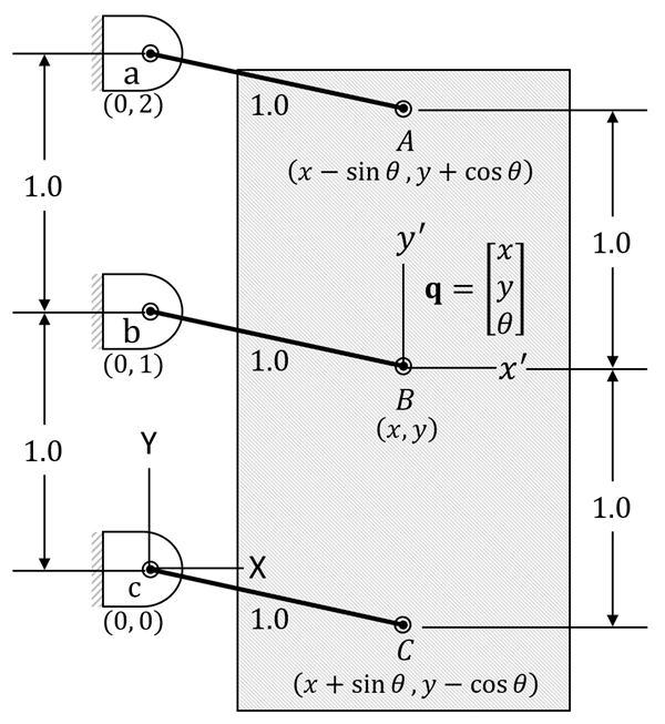
Consider a system where a rigid body has three points, A, B, and C, connected
to fixed ground points a, b, and c by inextensible links, each of length 1. The
generalized coordinates  describe the position and orientation of the body at point B
relative to the inertial reference frame. Points A and C are positioned based on
the rigid body's rotation, as shown in Figure 2.23: Example of Redundant Constraints.
describe the position and orientation of the body at point B
relative to the inertial reference frame. Points A and C are positioned based on
the rigid body's rotation, as shown in Figure 2.23: Example of Redundant Constraints.
The kinematic constraint equation  , ensuring that the distances between points A-a, B-b, and C-c
remain 1, is written as:
, ensuring that the distances between points A-a, B-b, and C-c
remain 1, is written as:
 | (2–177) |
The Jacobian matrix is derived by taking the partial derivatives of the constraint equations with respect to the generalized coordinates q. It is expressed as:
 | (2–178) |
At the initial state where θ=0, the above matrix simplifies to:
 | (2–179) |
By examining the simplified Jacobian matrix, you can observe that the third row is linearly dependent, as it can be generated by multiplying the first row by -1 and adding twice the second row. This reveals a redundant constraint. Since one of the constraints does not provide unique information about the system's motion, it can be eliminated. This redundancy simplifies the model by reducing the number of effective constraints.
The degrees of freedom of the system are calculated as follows:
 | (2–180) |
In this example, there are three generalized coordinates: x, y, and θ. After eliminating the redundant constraint, two independent constraints remain. Therefore, the degrees of freedom are 3 - 2 = 1. This indicates that the system has one degree of freedom, meaning it can move freely in one specific manner while satisfying the remaining constraints.
Note:
To avoid problems with redundant constraints, where forces are not distributed across multiple hinges but are concentrated in a single hinge, you can model force elements such as bushings instead of using hinges. Enter a high stiffness value in the direction where you want to constrain, and set the stiffness to zero in the direction where you don't want to constrain.
Joints implemented with Penalty-Based Constraints are not identified as redundant constraints. Although these joints may be redundantly connected within the system, they exhibit deformation, and the loads are distributed accordingly. This behavior distinguishes them from true redundant constraints, as the penalty-based approach allows for relative movement and load sharing between the connected elements.
Redundant constraint analysis is a series of processes that identify and resolve over-constraints in a system. This process not only simplifies calculations but also improves computational efficiency, especially when computational resources are important for complex systems modeled for dynamic simulations. The reduced system is optimized for faster processing and analysis while maintaining all necessary physical constraints.
This process is performed at each initial analysis stage, such as position, velocity, and acceleration analysis, and at the beginning of each analysis type, including static, dynamic, eigenvalue, and thermal analysis. Except for certain cases, redundant constraints identified in each analysis are removed only for that specific analysis, and new redundant constraints are identified in subsequent analyses.
In the position and velocity analysis, initial conditions for position and velocity are treated as constraints, and redundant constraints can be identified differently at each stage. Redundant constraints identified in the position and velocity analysis stages are removed only in each respective analysis and are re-initialized in the next analysis stage. For example, redundant constraints identified in the position analysis stage are removed only in position analysis, and new redundant constraints are identified in the velocity analysis stage.
Additionally, in the velocity analysis, the redundancy of initial velocities applied to each body is identified. If there is a conflict among the initial velocities applied to multiple bodies, some initial velocities may be removed as redundant and may not be reflected in the analysis.
If dynamic analysis follows acceleration analysis, no separate redundant constraint analysis is performed in the dynamic analysis. Instead, the redundant constraints identified in the acceleration analysis are used. If the acceleration analysis is skipped, redundant constraint analysis is performed during the dynamic analysis.
For static, eigenvalue, and thermal analyses, redundant constraint analysis is performed independently in each analysis.
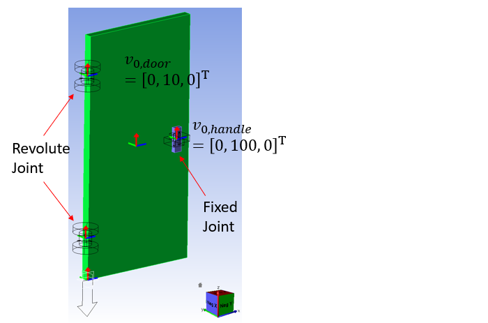
Example of Redundant Constraint Analysis in Motion
Consider a simple example to understand the identification and removal of redundant constraints in Motion. The figure below illustrates a simplified model of a door and a handle, both modeled as rigid bodies. Two revolute joints correspond to the hinges, and the door and handle are connected by a fixed joint. This is a perfect example of a redundant joint because the two revolute joints are modeled between the same two bodies, the ground and the door body, along the same rotational axis.
When redundant constraints exist, the message file outputs information about the redundant constraints identified and removed in each analysis. The figure below shows an excerpt of messages related to a redundant constraints analysis performed on a position, velocity, and acceleration analysis.
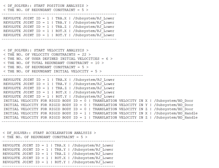
The message file includes the number of redundant constraints, the type of joint where the constraints were found, the constrained direction, and the name of the joint. The constrained direction is based on the joint's local coordinate system. It can be seen that redundant constraint analysis was performed at the position, velocity, and acceleration analysis stages, and the constraint of the revolute joint located below was removed. In joints where constraints are removed, no reaction force occurs, so it should be noted that the reaction force is reported as zero in the postprocessor.
In the case of velocity analysis, unlike other analyses, redundant initial velocities are additionally identified and removed. It can be seen that the initial velocity in the Y-direction of the handle is removed, while the initial velocity in the Y-direction of the door is not removed. Therefore, the initial velocities of the bodies in the Y-direction will be calculated based on the initial velocity applied to the door.
If the acceleration analysis proceeds normally, redundant constraint analysis is not performed in the subsequent dynamic analysis. Therefore, to verify which constraints were actually removed in the dynamic analysis, you should check the redundant constraints identified in the acceleration analysis.
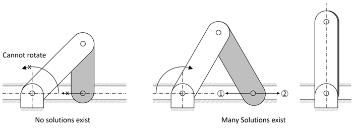
Singular configuration in a multibody system occurs when the constraint equations lead to a Jacobian matrix that is linearly dependent. These conditions present configurations where the system’s normal operation is disrupted because there are either multiple solutions for motion continuity or no feasible solutions at all. Such configurations challenge the predictability of the system characterized by the indeterminate or overly-constrained nature of the governing equations.
During analysis, if singularities occur, the Motion solver may fail to converge on a solution or may show unpredictability with even slight changes in conditions. Caution is therefore required. By understanding the specific conditions that lead to singularities, engineers can sidestep related complications. They can also refine the system's design by implementing adjustments, such as optimizing joint positions or altering the motion range. Such enhancements not only boost the system's efficiency but also avert potential operational issues.