


Time integration methods are numerical techniques used to solve differential equations derived from the equations of motion of multibody systems. This section covers the numerical methods used for time integration in solving equations of motion, with a focus on both explicit and implicit methods, and discusses their stability and accuracy characteristics. The Motion Solver employs the generalized-alpha method for dynamic analysis, which is based on the implicit method. Understanding the explicit method, which is simpler, will aid in comprehending the implicit method.
The explicit time integration method determines the future state of a system based on its current state without the need to simultaneously solve algebraic equations. This method's foremost benefit lies in its straightforwardness and simplicity of implementation. It also facilitates efficient parallel processing. However, explicit methods typically necessitate small time steps to ensure stability, particularly with stiff equations. Consequently, they are particularly effective for closely monitoring short-duration events, such as collisions, but less suited for long-term analyses.
The explicit (forward) Euler method is a straightforward time integration method used to approximate the future state of a system. The Taylor expansion of an integration variable in the time domain can be written as:
 | (2–181) |
 | (2–182) |
where:
 = time step = time step |
 = state at n-th step = state at n-th step |
 = state at (n+1)-th step = state at (n+1)-th step |
 = first derivative of the state with respect to time at
n-th step = first derivative of the state with respect to time at
n-th step |
 = second derivative of the state with respect to time at
n-th step = second derivative of the state with respect to time at
n-th step |
The second-order Euler integration method involves truncating all terms after the third term. This is because the magnitude of the third term is much larger than the other truncation terms. As a result, the integration error of the second-order Euler method is approximated by the third-order term. The truncation error is:
 | (2–183) |
where:
 = truncation error = truncation error |
 = user-defined error tolerance = user-defined error tolerance |
To ensure the truncation error is below the user-specified tolerance, estimate the allowable integration step size using the following formula:
 | (2–184) |
where:
 = allowable integration step size = allowable integration step size |
 = third derivative of the state with respect to time at
n-th step = third derivative of the state with respect to time at
n-th step |
The truncation error's third time derivative can be estimated by calculating the divided difference between the second time derivatives before and after a time increment.
Stability of Explicit Euler Methods
It is impossible to investigate the stability properties of the Euler method for
general nonlinear differential equations comprehensively. We will therefore discuss
the stability properties of the Euler method for a simple linear differential
equation, specifically  .
.
The stability properties of the Euler method when applied to general differential equations can be predicted by locally linearizing the original problems. This process yields a corresponding simple linear differential equation. The numerical solution, after n steps, of the given simple linear differential equation can be obtained as follows:
 | (2–185) |
Since the final solution must converge to the exact solution, which is zero, after a sufficient number of steps.
 | (2–186) |
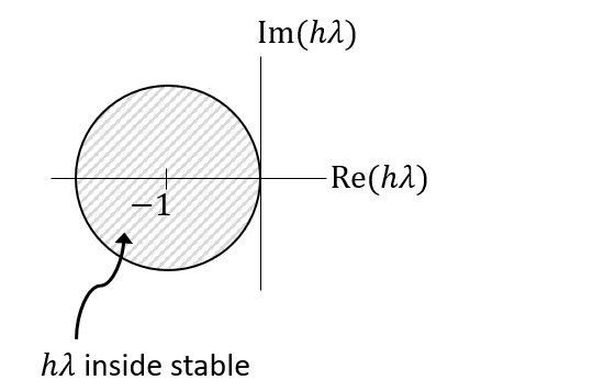
Thus, the factor 1+hλ must be less than 1.
 | (2–187) |
This convergence condition delineates the stability region, requiring that the values of 1+hλ lie within the unit circle in the complex plane. The stable step size can be determined for each λ value.
Below is a description of each step in the numerical integration process using the explicit method.
- Step 1: Initial Conditions Setup
At the initial time step (time=0), the system's state is defined by setting the initial values for position
 and velocity
  . These initial conditions are crucial as they
serve as the starting point for the numerical integration
process.
. These initial conditions are crucial as they
serve as the starting point for the numerical integration
process.- Step 2: Solving Equations of Motion
With the initial conditions set, the next step involves solving the system's equations of motion to determine the initial accelerations
 and any required Lagrange multipliers
λ. The equations of motion are typically
derived from the system's dynamic equations and constraints, forming
an augmented system that incorporates both the dynamic behavior and
the constraints imposed on the system.
and any required Lagrange multipliers
λ. The equations of motion are typically
derived from the system's dynamic equations and constraints, forming
an augmented system that incorporates both the dynamic behavior and
the constraints imposed on the system.- Step 3: Time Integration
The core of the explicit method lies in the numerical integration of the state variables, position and velocity, over time. Utilizing the explicit Euler method for numerical integration proceeds as follows.

(2–188)

(2–189)
- Step 4: Time Incrementation
After updating the position and velocity for the current time step, the time t is incremented by the step size h, moving the simulation forward in time.
- Step 5: Iteration
The process from steps 2 to 4 is repeated iteratively. In each iteration, the equations of motion are solved using the most recent state of the system (current positions and velocities) to find the new accelerations and Lagrange multipliers. The state variables are then updated using the numerical integration step, and time is advanced by h. This iterative process continues until the end of the simulation time is reached.
Unlike explicit methods, implicit methods such as the implicit Euler method update the system's state by implicitly solving a set of algebraic equations at each time step. These methods are notably more stable, particularly for stiff equations, and can operate effectively with larger time steps. This stability comes at the cost of increased computational effort due to the necessity of solving algebraic equations at each step.
In the implicit (Backward) Euler method, the
next state  is predicted by using
  and
and  , which involves the current and future states. This
requirement forms a fundamental part of the implicit method:
, which involves the current and future states. This
requirement forms a fundamental part of the implicit method:
 | (2–190) |
 | (2–191) |
where:
 = first derivative of the state with respect to time
at (n+1)th step = first derivative of the state with respect to time
at (n+1)th step |
| =
second derivative of the state with respect to time at
(n+1)th step |
This equation does not explicitly solve for and
therefore requires rearrangement and solving through numerical methods like
Newton's method. The need to use the state at the
(n+1)th step to compute itself introduces a
truncation error characteristic of implicit methods, which, while typically
smaller per step compared to explicit methods, involves more complex
calculations.
The truncation error  and allowable step size for implicit Euler method are
calculated from and its
Taylor series expansions as follows:
and allowable step size for implicit Euler method are
calculated from and its
Taylor series expansions as follows:
 | (2–192) |
Therefore,
 | (2–193) |
 | (2–194) |
where:
 | (2–195) |
 | (2–196) |
Stability of Implicit Euler Methods
Using the same approach as described for the stability of explicit methods, we
discuss the stability characteristics of the implicit Euler method for the
differential equation  .
.
The numerical solution of the given simple linear differential equation, after n steps, can be obtained using the implicit Euler method as follows:
 | (2–197) |
Since the final solution must converge to the exact solution, which is zero, after a sufficient number of steps.
 | (2–198) |
The final solution must converge to zero after sufficient steps, so the factor  must be less than 1.
 | (2–199) |
This condition is satisfied by any positive h. We therefore consider the implicit Euler method to be absolutely stable, regardless of the step size.
Below is a description of each step in the numerical integration process using the implicit method.
- Step 1: Initialization of the Implicit Method
At time = 0, solve for
 from the equations of motion using the given
initial conditions for position (
from the equations of motion using the given
initial conditions for position ( ) and velocity (
 ). When considering systems that include
constraint equations, the augmented equations of motion are
represented as:
). When considering systems that include
constraint equations, the augmented equations of motion are
represented as:
(2–200)
where:
 = mass matrix
 = second time derivatives of the
generalized coordinates
= second time derivatives of the
generalized coordinates = Jacobian matrix of constraints is
the derivative of the constraint equations with respect
to the generalized coordinates
= Jacobian matrix of constraints is
the derivative of the constraint equations with respect
to the generalized coordinates = Lagrange multipliers
 = generalized force
 = right-hand side of the constraint
equations
= right-hand side of the constraint
equations- Step 2: Initial Guess
update time t by the step size h
set initial guesses for
 ,
,  ,
,  and
and 
Calculate residuals


(2–201)

(2–202)

(2–203)

(2–204)
- Step 3: Newton's Method for Nonlinear Systems
Construct the Jacobian matrix
 of partial derivatives of the residuals
  with respect to
  ,
,  ,
,  and as follows:
(2–205)
where:


- Step 4: Iteration of Newton's Method
Solve the following matrix equation to find updates
 ,
,  ,
,  and
and  .
.
(2–206)
Update the guesses
 ,
,  ,
,  and
and  :
:
(2–207)
Repeat this step until convergence is achieved within a specified tolerance. If the solution does not converge despite continued iterations, reduce h and return to step 2.
- Step 5: Iteration
Repeat steps 2 through 4 until the desired simulation end time is reached.