


This section describes the constraints and boundary conditions that apply to nodal flexible bodies.
The Rigid Body Element (RBE) is a method for abstracting connections in a flexible body, also referred to as a Remote Boundary Condition. It defines constraints among nodes within a specified set. RBE is used to distribute applied loads and connect to other RBEs or rigid bodies through connectors such as joints or bushings.
Geometry Behaviors
Motion supports two geometry behaviors for RBE:
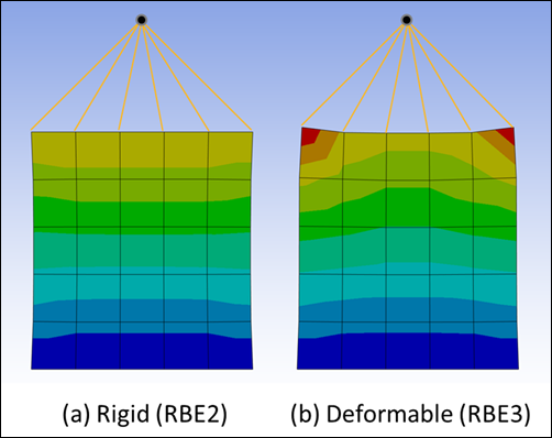
Rigid (RBE2): This behavior prevents any deformation within the connected nodes, maintaining a rigid structure. It is used when the connected elements need to move as a single, solid entity. This results in faster and more stable analysis compared to RBE3. It is recommended to use RBE2 if the area to be modeled with an RBE has high stiffness or is not the primary focus of the analysis. Additionally, RBE2 can be used to treat certain areas as rigid.
Deformable (RBE3): This behavior allows for controlled deformation, distributing applied loads more realistically and evenly across the connected nodes. It provides a flexible connection that can adapt to varying load conditions and deformations. Although analysis performance may be slower compared to RBE2, it offers more realistic modeling. For NVH (Noise, Vibration, and Harshness) issues, using RBE3 to model connecting elements in the force and vibration transmission path can yield more accurate results.
For formulations related to each geometry behavior, refer to sections Formulation of RBE2 (Rigid Type of Remote Boundary Condition) and Formulation of RBE3 (Deformable Type of Remote Boundary Condition).
Independent Node and Dependent Node
An RBE comprises an independent node (master node) and one or more dependent nodes (slave nodes). The dependent nodes are structural nodes located on a user-defined face or line and belong to an element. The independent node, typically a six-degree-of-freedom node generated by the preprocessor, is usually not part of any element. During Body Eigenvalue Analysis for generating modal data, this independent node serves as an interface node.
Creation of a Rigid Body Element
Motion Standalone Preprocessor: an RBE can be created by importing external FE data that includes an RBE or by generating a Nodeset. If the option to treat the Nodeset as an RBE is enabled in the Nodeset properties, the Nodeset is explicitly treated as an RBE, allowing you to directly determine the position of the independent node and select the geometry behavior. If this option is not enabled, the Nodeset is automatically treated as an RBE2 when a joint or vector force is connected, with the reference frame location of the joint or force set as the reference frame of the independent node. If nothing is connected to the Nodeset, it is ignored in the analysis. For detailed instructions on creating the Nodeset refer to the Nodeset section in the Motion Preprocessor User's Guide.
Mechanical Motion: an RBE can be created by generating a Remote Point, allowing you to directly determine the position of the independent node and select the geometry behavior. Additionally, when a joint or vector force is connected to a part of a flexible body (such as a surface or edge), an RBE is automatically generated for the nodes within the connected surface or edge. In this case, the location where the joint or force is connected will be set as the position of the independent node. For detailed instructions on creating Remote Points, refer to the Remote Points section in the Mechanical User's Guide.
Note: Concentrated load and pressure load do not automatically generate an RBE.
The RBE2, also known as the rigid type of remote boundary condition, models a fully rigid connection between the independent node and one or more dependent nodes. Forces and moments applied to the independent node are transmitted to the dependent nodes, treating all nodes as a single rigid body with no relative deformation between them.
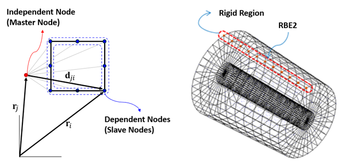
The relative displacement of a node in the RBE can be calculated from the independent node as follows:
 | (5–135) |
where:
| ri = position of the dependent node |
| rj = position of the independent node |
The displacement can be measured in the independent node's reference frame as follows:
 | (5–136) |
where:
| Aj = orientation matrix of the independent node reference frame |
Finally, the rigid region can be defined by the following constraint equation:
 | (5–137) |
where:
 = initial relative displacement = initial relative displacement |
The constraint force is calculated using the penalty method. For details on how to calculate the penalty force, refer to the Penalty-Based Constraints. The penalty stiffness of RBE2, determined internally, is based on the element stiffness and is set to a value significantly higher than the element stiffness, ensuring that RBE2 remains a relatively rigid region.
Note: Note that if a force significantly greater than the element stiffness is applied to the RBE2, some deformation may occur.
RBE3, also known as the deformable type of remote boundary condition, allows controlled deformation between nodes and distributes the loads (forces and moments) applied to the independent node among the dependent nodes. In contrast to the RBE2, which treats the connection as a fully rigid link, RBE3 provides flexibility in the connection.
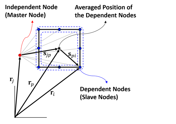
The average position of the dependent nodes is calculated as follows:
 | (5–138) |
where:
| rp = averaged position of the dependent nodes |
| ri = ith dependent node position |
| n = number of dependent nodes |
This can be expressed in terms of the relative displacement to the independent node:
 | (5–139) |
where:
| rj = position of the independent node |
| Aj = averaged orientation matrix of the dependent nodes |
| s′jp = relative displacement between independent node position and averaged position of the dependent nodes with respect to the dependent node's reference frame and is: |
 | (5–140) |
The constraint equations for RBE3 are derived from the condition that the sum of the differences between the initial average position of the dependent nodes and the position of each dependent node must remain constant even in the deformed state. The constraint equations for RBE3 are:
 | (5–141) |
where:
| s′pi = relative displacement between averaged position of the dependent nodes and i-th dependent node position with respect to the dependent node's reference frame and is: |
 | (5–142) |
Unlike RBE2, which is implemented using the penalty method, RBE3 utilizes the Lagrange Multiplier Method for its implementation.
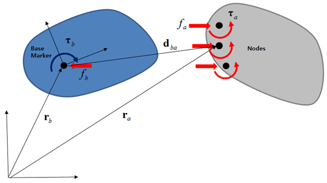
A Boundary Condition constrains the user-specified translational or rotational DOFs of one body relative to another body. A set of constrained equations are created corresponding to the number of nodes in the Node set.
For the rigid condition, the constraint equations at the position level of a node can be represented by the following equations:
 | (5–143) |
 | (5–144) |
where the vectors  and
and  ,
,  are the position of a node, and the absolute displacement and
orientation of the base markers, respectively.
are the position of a node, and the absolute displacement and
orientation of the base markers, respectively.  and
and  are the relative displacement between the node and base marker and
the orientation at the initial time. The unit vectors
are the relative displacement between the node and base marker and
the orientation at the initial time. The unit vectors  ,
,  ,
,  ,
,  ,
,  and
and  are the x, y and z-axes of the base marker and node,
respectively.
are the x, y and z-axes of the base marker and node,
respectively.
The constrained forces are defined from Lagrange multipliers and can be written as follows.
 | (5–145) |
The action force is applied to the node and an equal and opposite reaction force is applied and accumulated to the base marker.
 | (5–146) |
 | (5–147) |