


As shown in the figure below, the Relative error, Solver type, and several other parameters for the simulation can be defined in the solver tab of simulation configuration dialog. The parameters are described in the table below.
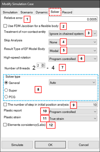
Figure 9.20: Solver parameters in the simulation configuration
| Feature | Description | Dimension (Range) | |||||||||||||||
| 1. Relative error | Use to define the relative error for the analysis. As the error is decreased, the accuracy of the analysis is increased. |
N/A (Real>0.0) | |||||||||||||||
| 2. Use FDM… | When this option is selected, the Jacobian matrix is calculated by FDM. When this option is not selected, the matrix is calculated analytically. If a nodal flexible body with beam or shell element is largely deformed, this option may improve the solving speed. | N/A | |||||||||||||||
| 3. Treatment of non-contact entity | Use to set a treatment method for non-contacted entities. This option helps to increase solver speed when there are many non-contacted entities, such as with a chain, belt, or tracked vehicle system. There are three options - , , and . For , when the model has a placing entity, the actually-contacted entities of all contact entities in the model are evaluated in the matrix calculation. For , when the model has more than one contact entity, the actually-contacted entities of all contact entities in the model are evaluated in the matrix calculation. For , all contact entities are evaluated in the matrix calculation. | N/A | |||||||||||||||
| 4. Skip Analysis | Use to skip initial analysis such as position, velocity and acceleration analysis. Initial analysis occasionally takes a long time, or may fail while displaying a memory overflow error. In these cases, this option is very helpful to shorten the simulation time or go to straight to dynamics or statics analysis by skipping the routines for the initial analysis. This field has four options - , , , and . For , the initial analysis is normally carried out. For , the position, velocity and acceleration analyses are ignored. For , the position and velocity analyses are ignored. For , the acceleration analysis is ignored. If the acceleration analysis is ignored, the initial acceleration error may become large. In this case, the initial step size must be set to a smaller value than the default value. For example, an initial step size of 1.0e-6 is better than the default value of 1.0e-4. | N/A | |||||||||||||||
| 5. Result Type of EF Modal Body |
Use to select the recording result type for an EasyFlex Modal body as or . The table below shows the differences the recording types.
| ||||||||||||||||
| 6. High-speed Rotation |
This property, applicable to high-speed rotation of nodal flexible bodies, determines whether the solver uses the orientation of the nodal body reference frame when calculating the position, velocity, and acceleration of nodes. Set High-speed Rotation to if you expect high-speed rotation of the nodal flexible body. For the solver type, High-speed Rotation is always Yes and the selected option is ignored. This property instructs the solver how to handle such an instance. Options include:
| N/A | |||||||||||||||
| 7. Number of threads | Use to define the power to calculate the number of threads for shared-memory parallel processing. The number of threads is calculated as 2^n. |
N/A (Integer>0) | |||||||||||||||
| 8. Solver type | Use to select a solver type to General, Super or PCG. The General solver is a solver for the general nonlinear equation of motion. This solver has three further options - , and . For the option, the solver automatically chooses an appropriate linear solver for a model. For , the required memory is minimized. For , the solving speed is faster than that of . As with the General solver, the Super solver is a solver for the nonlinear equation of motion but its solving speed is superior for problems without discontinuous contact. PCG (Preconditioned Conjugate Gradients) is an iteration solver, which is a faster solver than the above nonlinear solvers. PCG supports only FE Nodal Flex bodies. If EasyFlex bodies are included or modeled only as rigid bodies, PCG cannot be used. The PCG solver is generally good for large scale problems greater than approxiamtely100,000 D.O.F. | N/A | |||||||||||||||
| 9. The number of step… | Use to activate multiple steps for position analysis and to specify the number of steps used. When the initial condition of a joint is large, it is not possible to quickly find the initial position due to the local convergence of the Newton-Raphson Method. Position analysis must therefore be carried out several times, as defined in this field, using small increments of the large initial condition value. |
N/A (Integer>0) | |||||||||||||||
| 10. Plastic Report | Stresses and strains at nodes are reported either as values at gaussian points or as extrapolated values. For a plastic material in the elastic range, the option will report extrapolated values. For plastic material models, the values will be reported at the gaussian points for the plastic increment of the deformation. | N/A | |||||||||||||||
| 11. Plastic Strain | When models contain plastic material, you can select either or . | N/A | |||||||||||||||
| 12. Elements consistency(Labs) | This feature allows the solution of solid elements to return equivalent results to the MAPDL (Mechanical APDL) solver. When this option is enabled, it provides the same solution as when using the default settings for the MAPDL solver in analyses such as Static Structure or Transient Structure. This option is applicable to solid elements with isotropic and orthotropic materials. To utilize this option, you must select Elements Consistency in the program Setting > Labs section. | N/A |