3.2.1. Simulation Results Using a Contour

Various simulation results can be displayed by using the contour, as shown in the table below.

Figure 3.48: Simulation Results Using a Contour

Object	Mapping Type	Characteristics	Solution
Object	Mapping Type	Characteristics	Dynamics	Eigenvalue
FE & EF Body	Node (Averaged across body)	Displacement	O	X
		Velocity	O	X
		Acceleration	O	X
		Deformation	O	O
		Thermal	O	X
		Stress	O	X
		T Strain	O	X
		E Strain	O	X
		P Strain	O	X
		Top T Strain	O	X
		Top E Strain	O	X
		Top P Strain	O	X
		Bottom T Strain	O	X
		Bottom E Strain	O	X
		Bottom P Strain	O	X
		Contact	O	X
		Top Contact	O	X
		Bottom Contact	O	X
FE Body	Element (Unaveraged)	Stress	O	X
		T Strain	O	X
		E Strain	O	X
		P Strain	O	X
		Top T Strain	O	X
		Top E Strain	O	X
		Top P Strain	O	X
		Bottom T Strain	O	X
		Bottom E Strain	O	X
		Bottom P Strain	O	X
Rigid Body	Node (Averaged across body)	Contact	O	X
FE & EF Body	Element (Unaveraged)	Fatigue	O	X
FE & EF Body	Node (Unaveraged)	Top Stress	O	X
	Node (Unaveraged)	Top Strain	O	X
	Node (Averaged within material)	Top Stress	O	X
	Node (Averaged within material)	Top Strain	O	X
All Contacts	Contact	Pressure	O	X
		Normal Force	O	X
		Penetration	O	X
		DPenetration	O	X
		Friction Force	O	X
		Tangent Velocity	O	X
		Friction Coefficient	O	X
		Stiction Slip	O	X
		Slip Ratio	O	X
		Force Magnitude	O	X
		Spring Force	O	X
		Damping Force	O	X
		Potential Energy	O	X
		Contact Loss	O	X
		Sliding Loss	O	X
Beam Group	Beam Group	Displacement	O	X
		Velocity	O	X
		Acceleration	O	X
		Deformation	O	X
Chained System	Chained System	Tension Magnitude	O	X
		Tension Longitudinal	O	X
		Bending Loss	O	X
		Bending Loss Secondary	O	X
		Vibration Loss Tensile	O	X
		Vibration Loss Shear	O	X
		Vibration Loss Shear Scondary	O	X
		Slip Loss	O	X
		Stiction Slip	O	X
		Normal Force	O	X
		Penetration	O	X
		DPenetration	O	X
		Friction Force	O	X
		Tangent Velocity	O	X
		Friction Coefficent	O	X
User Subroutine	Ball Placing	Diameter	O	X
		Kinetic Energy	O	X
		Rotational Energy	O	X
	CVT	Penetration	O	X
		Penetration Dot	O	X
		Contact Stiffness	O	X
		Contact Damping Coefficient	O	X
		Normal Force	O	X
		Tangent Relative Velocity	O	X
		Tangent Friction Coefficient	O	X
		Tangent Friction Force	O	X
		Radial Relative Velocity	O	X
		Radial Friction Coefficient	O	X
		Radial Friction Force	O	X
		Contact Radius	O	X

3.2.1.1. Displacement

Displacement is used to display the displacement of nodes or a body and supports several components as shown in the table below.

Figure 3.49: Displacement in Contour

Component	Description
Magnitude	Magnitude of displacement vector
X	X component of displacement vector
Y	Y component of displacement vector
Z	Z component of displacement vector

3.2.1.2. Velocity

Velocity is used to display the translational velocity of nodes or a body and supports several components as shown in the table below.

Figure 3.50: Velocity in Contour

Component	Description
Magnitude	Magnitude of velocity vector
X	X component of velocity vector
Y	Y component of velocity vector
Z	Z component of velocity vector

3.2.1.3. Acceleration

Acceleration is used to display the translational acceleration of nodes or a body and supports several components as shown in the table below.

Figure 3.51: Acceleration in Contour

Component	Description
Magnitude	Magnitude of acceleration vector
X	X component of acceleration vector
Y	Y component of acceleration vector
Z	Z component of acceleration vector

3.2.1.4. Deformation

Deformation is used to display the translational and rotational deformations of nodes and supports several components as shown in the table below.

Figure 3.52: Deformation in Contour

Component	Description
Magnitude	Magnitude of deformation vector
X	X component of deformation vector
Y	Y component of deformation vector
Z	Z component of deformation vector
RM	Magnitude of rotational deformation
RX	X component of rotational deformation
RY	Y component of rotational deformation
RZ	Z component of rotational deformation

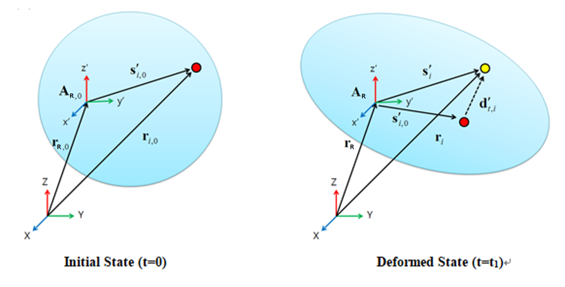
Definition of Deformation

The deformation vector is calculated with the difference between current position and initial position. If the reference frame is defined for the deformation, the deformation vector is transformed into the reference frame. At initial state and current state, the relative displacement vectors of a node relative to the center position can be defined by the following equations.

where, and are the nodal position vector and the position of the reference frame at initial time and is the orientation matrix of the reference frame. The deformation can be calculated with the relative displacement vectors as follows.

The vectors of and are the nodal position vector and the position of the reference frame at the current time, respectively.

The reference frame can be defined as the coordinate system in the flexible body.

Deformation scale () is derived as follows:

Where, and are the position of the reference marker and are , , scale values.

is Initial relative node position vector in Initial reference frame and is deformation vector of i-th node in deformed state.

3.2.1.5. Contact Results on Node

Contact is used to display the contact results on the contacted action nodes as shown in the table below. For shell elements, the contact results can also be reported in the direction of the top or bottom contact face.

Figure 3.53: Contact Results

Component	Description
Pressure	Used to display the pressure due to contact force. The pressure can be calculated from the elementary force divided by surface area of adjacent elements as follows. where, is the number of adjacent elements. The , , and are the elementary contact force, surface area of element and the number of nodes which belong to the element, respectively.
Normal Force	Use to display the contact normal forces. The force can be calculated as following equation. where , , and are the contact stiffness, damping coefficient, penetration and the first order time derivative of penetration, respectively.
Penetration	Use to display the contact penetration, which is equivalent to a deformation at the contact points in the normal direction. Note: According to Equation 6–19 in the Motion Theory Reference, contact penetration is calculated as negative by the solver, and negative contact penetration is reported with a positive sign to aid user comprehension.
DPenetration	Use to display the contact penetration velocity, which is equivalent to the first order time derivative of penetration. Note: According to Equation 6–54 in the Motion Theory Reference, contact penetration velocity that increases contact penetration is calculated as negative by the solver. In order to aid user comprehension and indicate penetration velocity that increases contact penetration with a positive sign, negative penetration velocity is reported.
Friction Force	Used to display the contact friction forces. The force can be calculated using the following equation. where, is the contact friction coefficient which is determined with user-defined friction coefficients and the tangential velocity.
Tangent Velocity	Used to display the tangential velocities, which are the relative velocities at the contact points in the tangential direction.
Friction Coefficient	Use to display the contact friction coefficients at contact points.
Stiction Slip	Used to display the stick-slip status at a contacted node. The stick-slip status can be represented as follows. 0: No contact. 1: Stiction. 2: Static (deformation is greater than the maximum stiction deformation and the tangential velocity is smaller than the stiction velocity). 3: Transient (tangential velocity is greater than the stiction velocity and smaller than the dynamics threshold velocity). 4: Dynamic (tangential velocity is greater than the dynamics threshold velocity).
Slip Ratio	Use to display the contact slip ratio at contact points.
Force Magnitude	Use to display the contact force at contact points as following equation. where is the contact force at each contact point. See Equation 6–46 in Intermittent Contact Force for more information.
Spring Force	Use to display the contact spring force at contact points as following equation.
Damping Force	Use to display the contact damping force at contact points as following equation.
Potential Energy	Use to display the potential energy due to contact as in the following equation: where is the exponent of penetration in Equation 6–52, is the contact spring force and is the contact penetration at the i^th contact point.
Contact Loss	Use to display the contact damping as following equation.
Sliding Loss	Use to display the friction force as following equation. where is the tangent velocity at the contact point.

Figure 3.54: Contact Component

Item	Description
Both	Used to display the contour results on the action and base geometry.
Base	Used to display the contour results on the base geometry.
Action	Used to display the contour results on the action geometry.

3.2.1.6. Thermal

Thermal is used to display the thermal results of nodes after the heat transfer analysis and supports several components as shown in the table below.

Figure 3.55: Thermal Results in Contour

Component	Description
Temperature	Temperature
Directional Heatflux X	X component of heat flux vector
Directional Heatflux Y	Y component of heat flux vector
Directional Heatflux Z	Z component of heat flux vector
Total Heatflux	Magnitude of heat flux vector
Thermal Strain	Thermal strain due to temperature change

3.2.1.7. Stress

Stress is used to display the nodal or elementary stress of FE and EF (EasyFlex) bodies and supports several components as shown in the table below. For an EF body, only nodal stress is available.

Figure 3.56: Stress Component

Component	Description
X	X component of normal stress,
Y	Y component of normal stress,
Z	Z component of normal stress,
XY	XY component of shear stress,
YZ	YZ component of shear stress,
ZX	ZX component of shear stress,
1^st Principal	Largest eigenvalue of stress tensor,
2^nd Principal	Middle eigenvalue of stress tensor,
3^rd Principal	Smallest eigenvalue of stress tensor,
Intensity
VonMises
Signed VonMises
Max Principal
Max Shear Stress

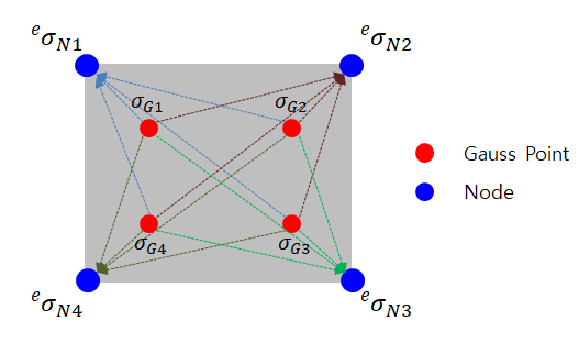
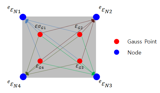
The stress is first calculated at the Gauss points of an element, and then they are extrapolated to get the nodal stress for each element as shown in the figure and equation below.

where, is the stress at the j^th Gauss point and is the i^th extrapolated nodal stress. is the number of nodes which belong to the element.

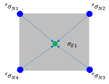
Figure 3.57: Extrapolated Nodal Stress

The element stress of the j^th element can be taken by averaging the stresses of nodes which belong to the element as shown in the figure and equation below.

Figure 3.58: Element Stress

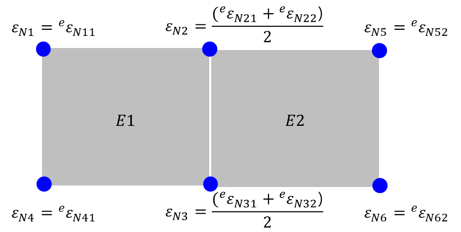
The node stress of i^th node can be taken by averaging the stresses of elements which contain the node as shown in the figure and equation below.

where, is the number of elements which include the i^th node.

Figure 3.59: Node Stress

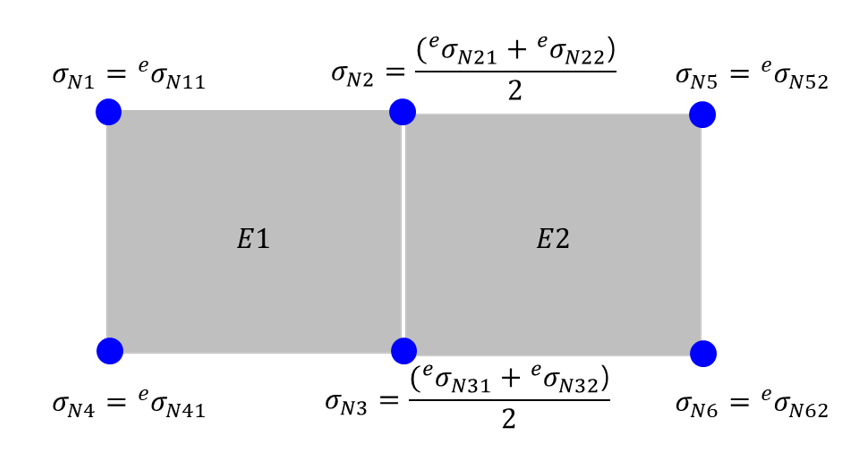
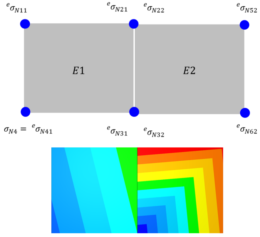
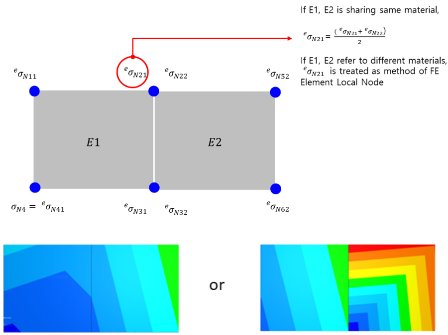
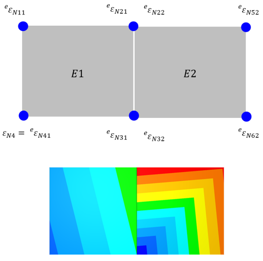
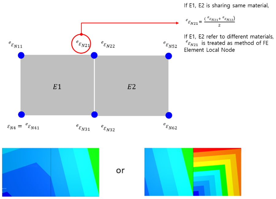
The element node is one of the mapping types for displaying the results from an element on a contour. The stress of i^th element node can be taken from local node stress of elements which contain the node. This is available for EF or FE bodies which refer to a linear material. Depending on the type of the method or condition, the equation can be different as shown in the figures below.

Figure 3.60: Node (Unaveraged)

Figure 3.61: Node (Averaged within material)

3.2.1.8. T Strain

T Strain is used to display the nodal or elementary strain of FE and EF (EasyFlex) bodies. T Strain means total strain, which can be calculated as the sum of elastic strain and plastic strain by following equation.

T Strain supports several components as shown in the table below. For an EF body, only nodal strain is available.

Figure 3.62: Strain Component

Component	Description
X	X component of normal strain,
Y	Y component of normal strain,
Z	Z component of normal strain,
XY	XY component of shear strain,
YZ	YZ component of shear strain,
ZX	ZX component of shear strain,
1^st Principal	Largest eigenvalue of strain tensor,
2^nd Principal	Middle eigenvalue of strain tensor,
3^rd Principal	Smallest eigenvalue of strain tensor,
Intensity
Von Mises

The strain can be calculated in the same way as stress. First, the strain is calculated at the Gauss points of an element, and then they are extrapolated to get the nodal strain for each element as shown in the figure and equation below.

where, is the strain at the j^th Gauss point and is the i^th extrapolated nodal strain. is the number of nodes which belong to the element.

Figure 3.63: Extrapolated Nodal Strain

The element strain of j^th element can be taken by averaging the strains of nodes which belong to the element as shown in the figure and equation below.

Figure 3.64: Element Strain

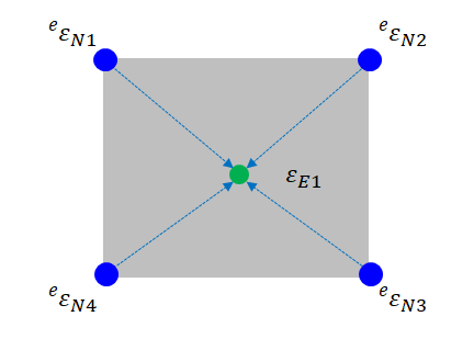
The node strain of i^th node can be taken by averaging the strains of elements which contain the node as shown in the figure and equation below.

where, is the number of elements which include the i^th node.

Figure 3.65: Node Strain

The element node is one of the mapping types for displaying the results from an element on a contour. The strain of i^th element node can be taken from the local node strain of elements which contain the node. This is available for EF or FE bodies refering to a linear material. Depending upon the type of the method or condition, the equation can be different as shown in the figure below.

Figure 3.66: Node (Unaveraged)

Figure 3.67: Node (Averaged within material)

3.2.1.9. E Strain

E Strain is used to display the elastic strain of nodes and elements, and supports several components (the same components as T Strain). For an EF body, only nodal strain is available.

3.2.1.10. P Strain

P Strain is used to display the plastic strain of nodes and elements by permanent deformation, and supports several components (the same components as T Strain). For an EF body, only nodal strain is available.

3.2.1.11. Fatigue

Fatigue is used to display the simulation results after fatigue analysis and supports several components as shown in the table below.

Figure 3.68: Fatigue Component

Component	Description
Life Cycle	Used to define the number of loading cycles that a body sustains before failure of a specified nature occurs.
Damage	Used to define the inverse of the life cycle. As the value becomes larger, the possibility of failure is increased.

3.2.1.12. Chained System

Chained System is used to display the simulation results of CPlacing and supports several characteristics as shown in the table below.

Figure 3.69: Chained System Characteristics

Characteristic	Description
Tension Magnitude	Used to display the average or sum of contact normal forces. The force can be calculated using the following equation. where ,, , and are the contact stiffness, damping coefficient, penetration and the first-order time derivative of penetration, respectively.
Tension Longitudinal	Used to display the average or sum of penetration which is equivalent to a deformation at the contact points in the normal direction.
Bending Loss	Used to display the loss due to the repeated bending deformation of a belt. The primary bending loss is calculated with the relative angular velocity in the z-axis of the segment using the following equation. where is the rotational damping coefficient and is the relative angular velocity between two adjacent segments in the z-axis.
Bending Loss Secondary	Used to display the loss due to the repeated bending deformation of a belt. The secondary bending loss is calculated with the relative angular velocity in the y-axis of a segment using the following equation. where is the rotational damping coefficient and is the relative angular velocity between two adjacent segments in the y-axis.
Vibration Loss Tensile	Used to display the loss by the vibration of a belt. The tensile vibration loss is the loss in the x-axis of a segment can be calculated using the following equation. where is the translational damping coefficient and is the relative velocity between two adjacent segments in the x-axis.
Vibration Loss Shear	Used to display the loss by the vibration of a belt. The primary shear vibration loss is the loss in the y-axis of a segment can be calculated using the following equation. where is the translational damping coefficient and is the relative velocity between two adjacent segments in the y-axis.
Vibration Loss Secondary	Used to display the loss by the vibration of a belt. The secondary shear vibration loss is the loss in the z-axis of segment can be calculated using the following equation. where is the translational damping coefficient and is the relative velocity between two adjacent segments in the z-axis.
Slip Loss	Used to display the frictional loss by the slip of bearing in the circumferential direction. The slip loss can be calculated using the following equation. where is the friction coefficient, is the magnitude of bearing forces on the radial plane, and is the relative velocity of the bearing in the circumferential direction.
Stiction Slip	Used to display the stick-slip status at a contacted node. The stick-slip status can be represented as follows. 0: No contact. 1: Stiction. 2: Static (deformation is greater than the maximum stiction deformation and the tangential velocity is smaller than the stiction velocity). 3: Transient (tangential velocity is greater than the stiction velocity and smaller than the dynamics threshold velocity). 4: Dynamic (tangential velocity is greater than the dynamics threshold velocity).
Slip Ratio	Used to display the average or sum of slip ratios at contact points.
Normal Force	Used to display the average or sum of contact normal forces. The force can be calculated using the following equation. where , , and are the contact stiffness, damping coefficient, penetration and the first-order time derivative of penetration, respectively.
Penetration	Used to display the average or sum of penetration, which is equivalent to a deformation at the contact points in the normal direction.
DPenetration	Used to display the average or sum of the first-order time derivative of penetration.
Fiction Force	Used to display the average or sum of contact friction forces. The force can be calculated using the following equation. where is the contact friction coefficient, which is determined with user-defined friction coefficients and the tangential velocity.
Tangent Velocity	Used to display the average or sum of tangential velocities, which are the relative velocities at the contact points in the tangential direction.
Friction Coefficient	Used to display the average or sum of friction coefficients at contact points.

Each characteristic of a chained system supports two components as shown in the table below.

Figure 3.70: Chained System Component

Characteristic	Description
Value	Used to display the values of simulation results.

3.2.1.13. CVT

CVT is used to display the simulation results of a CVT system and supports several characteristics as shown in the table below.

Figure 3.71: CVT System Characteristics

Characteristic	Description
Penetration	Used to display the penetration. It is the penetration between Pin and Pulley.
Penetration Dot	Used to display the first-order time derivative of penetration between Pin and Pulley. This value is 0 without contact.
Contact Stiffness	Used to display the contact stiffness. The contact stiffness can be calculated using following equation where , , and are the contact stiffness, string force and penetration.
Contact Damping Coefficient	Used to display the contact damping coefficient, which can be calculated using following equation where, and are the damping coefficient, damping force and the first order-time derivative of penetration.
Normal Force	Used to display the normal force.
Tangent Relative Velocity	Used to display the tangential relative velocity of Pin with respect to Pulley at the contact point.
Tangent Friction Coefficient	Used to display the tangential friction coefficient at the contact point.
Tangent Friction Force	Used to display the applied tangential friction force for Pin with respect to Pulley at the contact point.
Radial Relative Velocity	Used to display the radial relative velocity of Pin with respect to Pulley at the contact point.
Radial Friction Coefficient	Used to display the radial friction coefficient at the contact point.
Radial Friction Force	Use to display the applied radial friction force for Pin with respect to Pulley at the contact point.
Contact Radius	Use to display the contact radius. This is the minimum distance between the axis of rotation and the contact point.

3.2.1.14. Ball Placing

Ball Placing is used to display the simulation results of a system with many ball bearings and supports several characteristics as shown in the table below.

Figure 3.72: Ball Placing System Characteristics

Characteristic	Description
Diameter	Used to display the diameter of balls in Ball Placing entity.
Kinetic Energy	Used to display the kinetic energy of balls in Ball Placing entity. The kinetic energy can be calculated using following equation. where, m and v are the mass of the ball and velocity of the ball, respectively.
Rotational Energy	Used to display the rotational energy of balls in Ball Placing entity. The rotational energy can be calculated as following equation. where, J and are the mass moment of inertial of the ball and angular velocity of the ball, respectively.