


VM-LSDYNA-FLUID-004
VM-LSDYNA-FLUID-004
Unsteady 2D Laminar Flow around a cylinder in a Channel
Overview
| Reference: | Schafer, M. & Turek, S. (1998). Benchmark computations of laminar flow around a cylinder. In Hirschel, E. (Ed.), Flow simulation with high-performance computers II. Notes on numerical fluid mechanics (NNFM) (547–566). Herzog-Heinrich-Weg 6, D-85604, Zorneding, Federal Republic of Germany. |
| Analysis Type(s): | Incompressible CFD |
| Input Files: | Link to Input Files Download Page |
Test Case
This test case reproduces a two-dimensional, unsteady, incompressible laminar flow around a cylinder inside a channel. The purpose is to validate the maximum drag and lift force coefficients and the pressure difference between the front and end points of the cylinder.
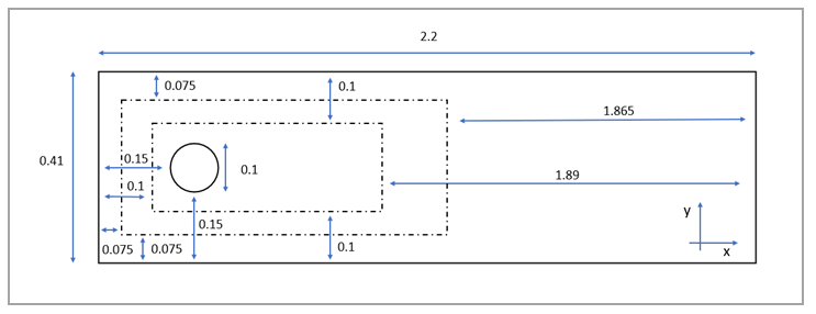
The domain consists of a rectangular box (the channel) with an inflow of prescribed velocity, an outflow of prescribed pressure, and the two remaining sides of the boundary (the channel's walls) with non-slip conditions. The cylinder also features a non-slip condition. The domain size and relevant quantities are shown in Figure 153. The cylinder location, as you can see, is not perfectly symmetrical with respect to the channel height. Two meshing boxes have been used to selectively refine the mesh around the cylinder and its wake.
For this test case, all units of measure are consistent (length = m, time = s, mass = kg, force = N, pressure = Pa).
| Material Properties | Geometric Properties | Loading |
|---|---|---|
|
Fluid: • Fluid density ρ = 1 • Inflow max velocity in channel’s axial direction Um = 1.5 • Flow dynamic viscosity μ = 10-3 |
Mesh Size: • Fluid boundaries elements size: 0.008 • Cylinder elements size: 0.0005 • Anisotropic elements added to cylinder Boundary Layer: 6 • Anisotropic elements added to channel Boundary Layer: 4
Geometry: • Cylinder Diameter D = 0.1 • Channel Height H = 0.41 |
Fluid: • Outflow pressure p = 0 |
Analysis Assumptions and Modeling Notes
The behavior of the flow is characterized by the Reynolds number:
 | (13) |
where ρ is the fluid's density, D is the characteristic length of the problem (that
is, the cylinder diameter), and μ is the dynamic viscosity of the flow.  is the flow mean velocity field at the channel's inlet:
 | (14) |
where U is the (unsteady) velocity field in the channel's axial direction which is imposed at the inlet (x = 0). The complete inflow velocity field relation is:
 | (15) |
Where  is the maximum inflow velocity in the channel's axial direction. This yields
a maximum Reynolds number
is the maximum inflow velocity in the channel's axial direction. This yields
a maximum Reynolds number  .
.
In this study, the time interval is  . The values of drag, and lift coefficients (respectively,
  and
and  ) will be plotted, and their maximum value (
 and
and  ) will be compared to the values in the reference.
Note that the nondimensional coefficients are evaluated using the following relation:
 | (16) |
where  is the maximum of
  for the considered time interval and
  is the relative dimensional force on the cylinder surface. It's important to
understand that the drag force is the resultant force on the cylinder in the asymptotic flow
direction (x direction), lift force is the resultant force on the cylinder orthogonal to the
asymptotic flow direction (y direction), and both forces are the sum of pressure and viscous
forces.
is the relative dimensional force on the cylinder surface. It's important to
understand that the drag force is the resultant force on the cylinder in the asymptotic flow
direction (x direction), lift force is the resultant force on the cylinder orthogonal to the
asymptotic flow direction (y direction), and both forces are the sum of pressure and viscous
forces.
As a further reference value, the pressure difference
 is defined, with the front and end points of the cylinder,
  and
and  , respectively. Value
  will be compared to the same value in the reference.
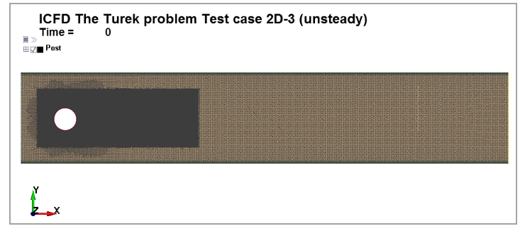
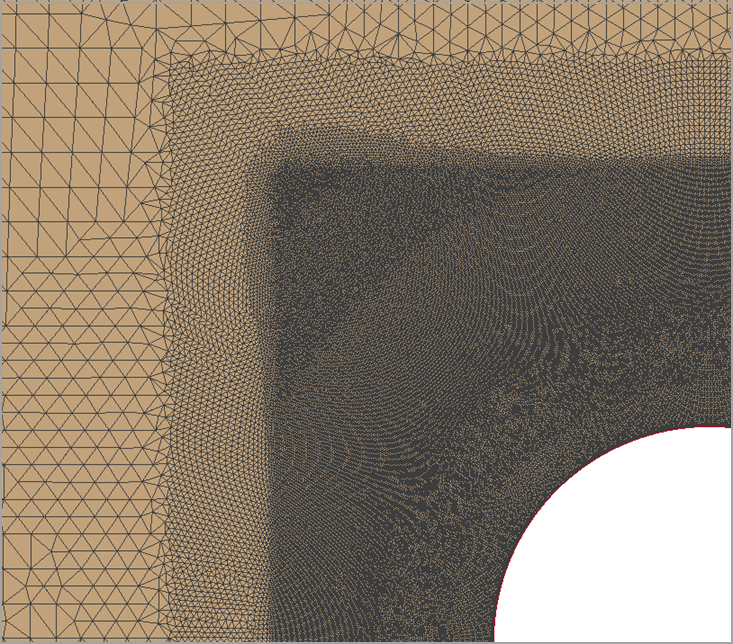
A picture of the domain's mesh is shown in Figure 154, while Figure 155 shows a detail of the mesh refinement around the cylinder and the channel's walls.
Results Comparison
Figure 156 shows the flow velocity contour in the channel's axial direction at different times. The development of unsteady vortices in the cylinder wake is evident.
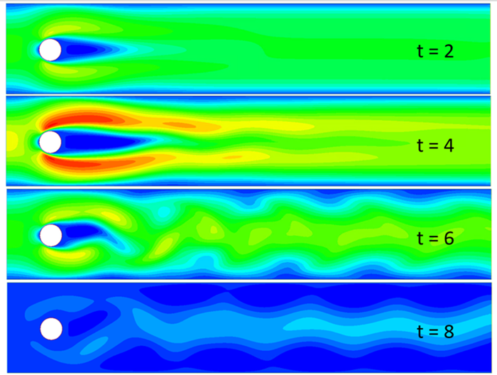
Figure 157 and Figure 158 show, respectively, the drag
and lift coefficients over time. The table below shows a comparison of the maximum drag and
lift coefficients ( and
and  ) and pressure difference
  between the present analysis and the reference. The reference proposes a
comparison of the same values calculated with a variety of different numerical methods. The
value shown below in the target column for each variable is the average between its upper and
lower bounds.
between the present analysis and the reference. The reference proposes a
comparison of the same values calculated with a variety of different numerical methods. The
value shown below in the target column for each variable is the average between its upper and
lower bounds.
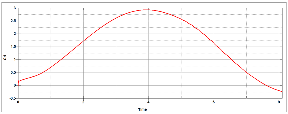
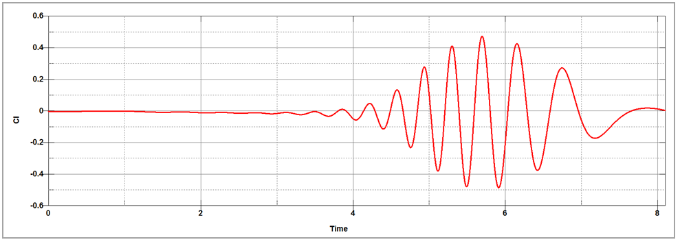
| Result | Target | LS-DYNA | Error (%) |
 | 2.9500 | 2.9399 | 0,34% |

| 0.4800 | 0.4760 | 0.83% |
 | - 0.1100 | -0.1118 | 1.63% |