

MAPDL LS-DYNA co-simulation utilizes the strength of Mechanical APDL and LS-DYNA solver technologies to improve the simulation solution stability and accuracy of complex problems. This chapter describes procedures to set up and run a Mechanical APDL and LS-DYNA co-simulation analysis to accurately capture the fluid structure interaction (FSI) of the reflow process and predict the final shape and location of solder balls on a printed circuit board (PCB).
Go to a section topic:
Overview
The reflow process is essential in semiconductor manufacturing for creating reliable connections in integrated circuit (IC) packaging. It involves melting and adhering solder balls to flux-coated pads to create permanent electrical connections on a PCB. Electrical and mechanical connections are made by melting solder balls placed on the substrate or chip pads and forming metallurgical bonds with the pads. As the assembly cools, the solder joints solidify to secure component placement. Undesired solder bonding is a common defect in IC packaging that negatively impacts the electrical performance and reliability of the chips. It can cause the circuit to malfunction or fail due to unintended electrical connections between components created by the solder balls.
Simulation tools can predict the final shape and location of solder balls, provide insight into the quality of IC packaging designs, and deliver accurate inputs for further electrical performance and reliability simulations. To accurately capture the fluid structure interaction (FSI) of the reflow process, an FSI solver is required. Instead of using a monolithic solver to solve the FSI problem, the existing, well-established fluid and structural solvers from various Ansys products are utilized in a domain-partitioned approach.
MAPDL LS-DYNA co-simulation combines the strengths of Mechanical APDL and LS-DYNA solver technologies to improve the simulation solution stability and accuracy of the reflow process. The Incompressible Smoothed Particle Galerkin (ISPG) solver in LS-DYNA is a Lagrange-based implicit solver for incompressible fluid which can track the free surfaces of solder balls. Mechanical APDL is an implicit structure solver with advanced reinforcing and embedding element technologies that can be used to perform accurate and efficient simulations that include PCB modeling. Both solvers have the capability to use Distributed-Memory Parallel (DMP) mode (known as Massively Parallel Processing (MPP) in LS-DYNA). The co-simulation feature utilizes a general coupling framework to support the FSI coupling of both solvers. The figure below shows a PCB and the domain, which includes the solder balls and substrate, that is simulated to demonstrate how to setup and run a Mechanical APDL LS-DYNA co-simulation analysis.

Using the Co-simulation Feature
To use the co-simulation feature:
Install Workbench/Mechanical version 2025 R1 or later, and activate the MAPDL LS-DYNA co-simulation beta feature .
Download the supported LS-DYNA solver using the following link and extract the files to your working directory:
Set up the model in the Mechanical application for the Mechanical APDL and LS-DYNA analyses.
Create the solver input files and setup files for Mechanical APDL and LS-DYNA.
Verify the postprocessing co-simulation results.
Activating the MAPDL LS-DYNA Co-simulation Beta Feature
To make the beta options available from Workbench:
On the Workbench project page, go to and then select the option Appearance.
Scroll down and activate the Beta Options check box.
Click .
Return to and select the option .
Scroll down to the LS-DYNA section, activate the Enable Writing Input Files for MAPDL LSDYNA Cosimulation check box.
Click .
Restart Workbench for the beta feature to take effect.
Open or return to Mechanical.
Setting up the Model in the Mechanical application
The Mechanical application provides an integrated environment to build the finite element FSI model between solder balls and PCBs, as shown in the figure below. The solder ball parts form the fluid domain of an LS-DYNA analysis with ISPG solver. Each solder ball is an individual part that can only be a regular tetrahedron element. The other parts of the assembly form the structure domain of the Mechanical APDL structure solver.

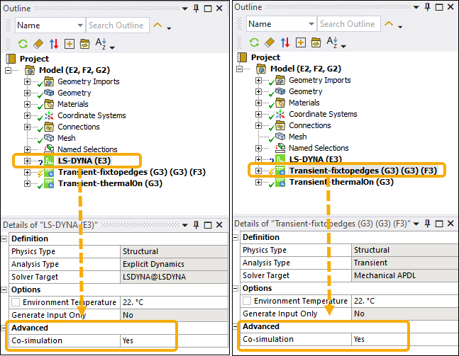
An MAPDL LS-DYNA co-simulation includes both a Mechanical APDL structural analysis and an LS-DYNA analysis system in any order. In the example below, the Transient-fixtopedges system is the Mechanical APDL structural analysis system. Specify the co-simulation as follows:
For each analysis system, set the Co-simulation property to Yes in the Details pane Advanced category.
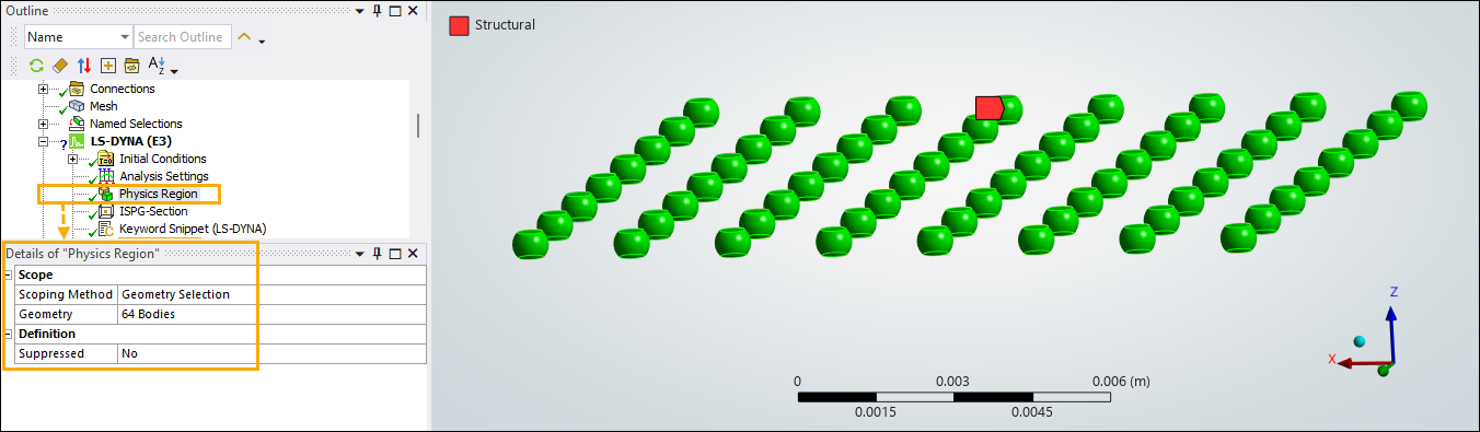
Define a Physics Region for each analysis system. The Physics Region for the LS-DYNA system is scoped to the solder balls only.
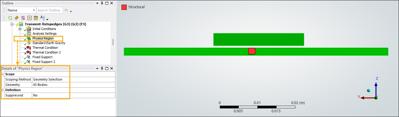
For the Mechanical APDL structural analysis system (Transient-fixtopedges), it is scoped to the substrates that are in contact with the solder balls.
Define the ISPG-Section properties for the LS-DYNA analysis system.
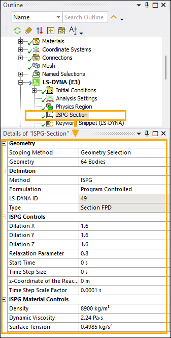
For details about *SECTION_SOLID_FPD, *MAT_IFPD, refer to Part Setup in the LS-DYNA User's Guide.
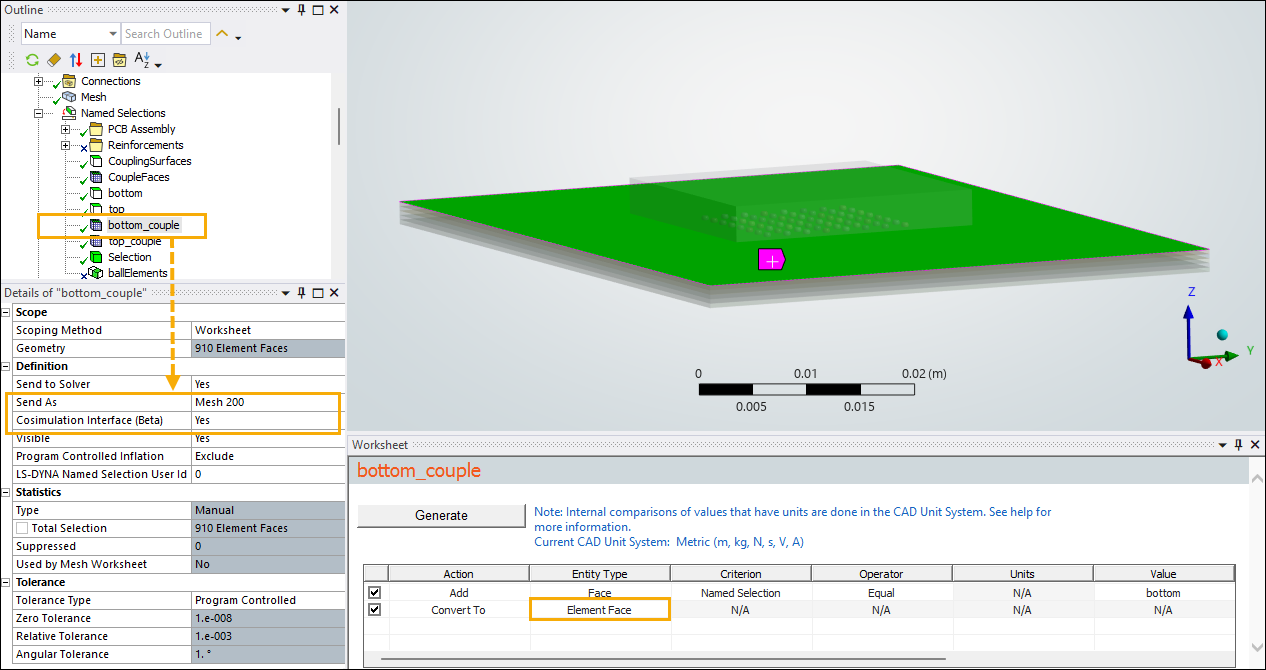
Use Named Selections to define the surfaces of the substrate that are in contact with the solder balls for the co-simulation. To do this:
Select the top surface of the bottom plate in the geometry window, right-click, choose , and name it “bottom_couple”. Repeat this for the bottom surface of the top plate and name it “top_couple”.
For each named selection, right-click it and select Create a Nodal Named Selection ("bottom_couple" and "top_couple" in the example below). From their worksheet, for the Convert To action, set Entity Type to Element Face and click to apply the changes. In the Details pane, under Definition, set Send As to Mesh 200 and Cosimulation Interface (Beta) to Yes (see figure below).
Insert an ISPG to Surface Coupling object and define the co-simulation interface coupling pairs for each contact surface specified in the previous step. For example, for the ISPG to Surface Coupling-bottom: scope the ISGP Part to the solder balls and scope the Surface using the “bottom_couple” Named Selection defined in the previous step (see figure below). ISPG to Surface Coupling-top is the same except its Surface is scoped to the “top_couple” Named Selection.

For more information about the ISPG to Surface Coupling object, refer to Setting up a Project in the LS-DYNA User's Guide.
Define all other loading, boundary conditions, and analysis settings for the Mechanical APDL solver by specifying object properties and/or command snippets entered in a command (APDL) object.
Use the CSOPT command in a command (APDL) object to specify solution options for a Mechanical APDL LS-DYNA co-simulation analysis.
Creating the Solver Input Files and Setup Files
After you have finished setting up the finite element model in the Mechanical application, create the solver input and setup files required for the co-simulation.
Create the input files for both solvers using the Mechanical application:
Select the Mechanical APDL analysis system, click , and save the APDL input file with a file name of your choice (for example, solidPCB.dat). The export creates one file.
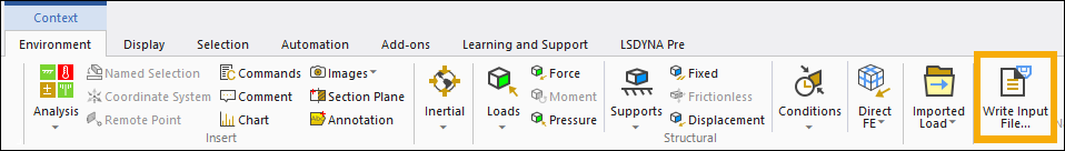
Select the LS-DYNA analysis system, click , and then save the LS-DYNA input file with a file name of your choice. The export creates two files (for example, LSDYNA_input_files.k and LSDYNA_INCLUDE_COSIM.k). The main input file contains the keyword *INCLUDE_COSIM which defines the co-simulation information.
Copy or move the input files to your working directory.
Create the setup *.txt files:
Create the Mechanical APDL co-simulation setup file (for example, apdlInput.txt).
The Mechanical APDL setup file requires the following two lines:
The first line specifies the Ansys Structure solver executable. Instead of specifying the full path to the executable,
ansys.ecan be used and the program uses the installed 2025 R1 release version automatically.The second line specifies all the command line arguments for the structural solver, where:
-stg 1must be included to start the co-simulation in Mechanical APDL. For information on command line options, see Starting a Mechanical APDL Session from the Command Level in the Operations Guide.
For example:
ansys.e
-stg 1 -b -i solidPCB.dat -o solve.out
Create a LS-DYNA co-simulation setup file (for example, dynaInput.txt).
The LS-DYNA setup file requires the following two lines:
The first line specifies the Ansys LS-DYNA MPP solver executable that was you had downloaded earlier. The full path of the executable is required.
The second line specifies all the command line arguments for the ISPG fluid flow solver, where:
ncsp=-1must be included in the setup file for the solver to start the co-simulation,i=specifies the input file, andp=defines an LS-DYNA pfile to control the MPP decomposition. Defining a pfile is optional.
For example:
D:/lsdyna_mpp_dp_impi_beta.exe
ncsp=-1 i=LSDYNA_input_files.k p=pfile64.txt
Note: To improve the MPP performance, the LS-DYNA solver requires each solder to be an individual part and is combined into one MPP node. This is controlled using the keyword *CONTROL_MPP_DECOMPOSITION_ARRANGE_PARTS, which is specified in the LS_DYNA input file (for example, LSDYNA_INCLUDE_COSIM.k) or an optional pfile.
Running the MAPDL LS-DYNA Co-simulation
From a shell terminal (Linux) or command-line prompt (Windows), go to your working directory and run the Mechanical APDL LS-DYNA co-simulation command:
ansys251 -csim -napdl np -ndyna np -apdl setupfile -dyna setupfile
Where:
-csim | Specifies a co-simulation run. |
-napdl np | Defines the number of processes for the Mechanical APDL solver. The default value is 2. |
-ndyna np | Defines the number of processes for the LS-DYNA solver. The default value is 2. |
-apdl setupfile | Specifies the name of the Mechanical APDL co-simulation setup file. If you
omit the |
-dyna setupfile | Specifies the name of the LS-DYNA co-simulation setup file. If you
omit the |
Postprocessing Co-simulation Results
Co-simulation yields two sets of results: one for the LS-DYNA ISPG fluid flow solver, and one for the Mechanical APDL structural solver. The Mechanical APDL GUI and LS-DYNA post-processing tools can be used to individually process each solver's output. For more postprocessing options for the Mechanical APDL results, refer to Writing and Reading the Mechanical APDL Application Files in the Mechanical User's Guide. For more postprocessing options for the LS-DYNA results, refer to Writing and Reading the LS-DYNA Application Files in the Mechanical User's Guide