Chapter 9: Performing Parametric Analyses in Ansys Fluent

This tutorial is divided into the following sections:

9.1. Introduction

This tutorial illustrates how to perform a parametric analysis, or study, of a static mixer simulation within Ansys Fluent. The analysis will take an existing Fluent case file with predefined input and output parameters, and setup and solve various permutations that analyze a few changes to the parametric variables, all within the Fluent interface. For more information about using Fluent to perform a parametric analysis, refer to Performing Parametric Studies.

This tutorial demonstrates how to do the following:

Start with a Fluent case and data file with input and output parameters.
Define a series of additional cases (design points) where each represents a change to one or more the parameters.
Update the series of design points.
Generate a simulation report for each design point.
Review the simulation reports and perform a comparison of the results between design points.

Related video that demonstrates steps for setting up, solving, and postprocessing a parametric study in Fluent:

9.2. Prerequisites

This tutorial is written with the assumption that you have completed one or more of the introductory tutorials (such as Fluid Flow and Heat Transfer in a Mixing Elbow) found in this manual and that you are familiar with the Ansys Fluent tree and ribbon structure. Some steps in the setup and solution procedure will not be shown explicitly.

9.3. Problem Description

The problem being analyzed involves a static mixer with two inlets and an outlet.

Figure 9.1: Problem Schematic

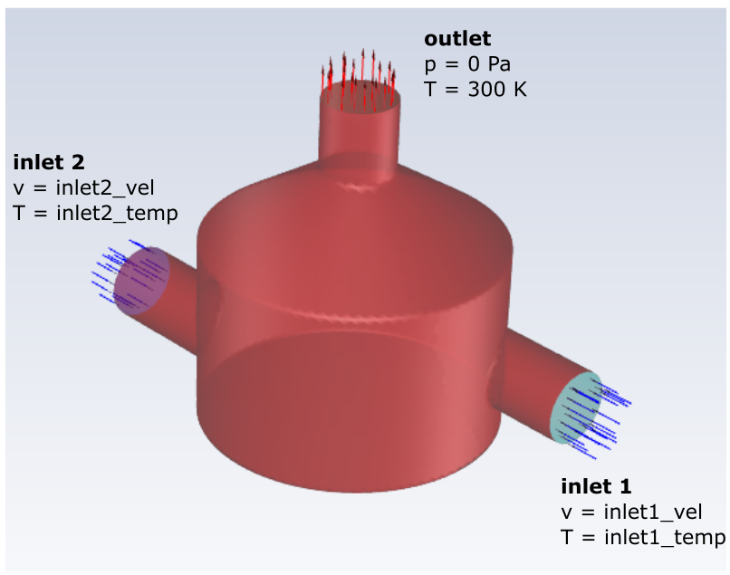
Fluid enters through two inlets using conditions described by separate input parameter expressions for the fluid velocity magnitude (inlet1_vel and inlet2_vel) and temperature (inlet1_temp and inlet2_temp). The fluid exits the outlet of the mixer based on a pressure outlet condition with a temperature of 300 Kelvin.

The input parameter expressions are initially set to the following constant values:

Input Parameter	Value
`inlet1_vel`	5 m/s
`inlet1_temp`	300 K
`inlet2_vel`	10 m/s
`inlet2_temp`	350 K

9.4. Setup and Solution

The following sections describe the setup and solution steps for this tutorial:

9.4.1. Preparation

To prepare for running this tutorial:

Download the parametric_mixer.zip file here .
Unzip parametric_mixer.zip to your working directory.
The files Static_Mixer.cas.h5 and Static_Mixer.dat.h5 can be found in the folder.
Use the Fluent Launcher to start Ansys Fluent.
Select Solution in the top-left selection list to start Fluent in Solution Mode.
Select 3D under Dimension.
Enable Double Precision under Options.
Set Solver Processes to 4 under Parallel (Local Machine).

9.4.2. Mesh

Read the case and data file (Static_Mixer.case.h5 and Static_Mixer.dat.h5).
File → Read → Case & Data...
As Fluent reads the case/data files, it will report the progress in the console.
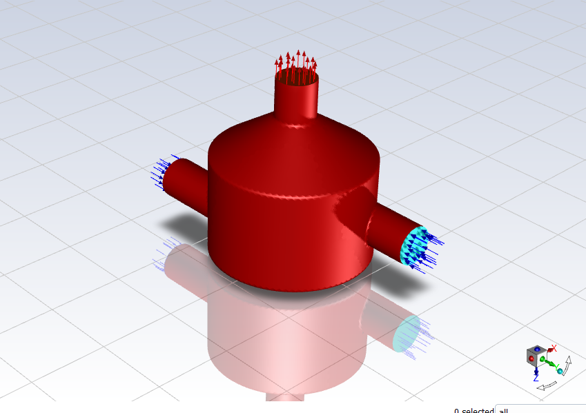
Examine the mesh (Figure 9.2: Mesh Display of the Static Mixer).
Note: You can use the right mouse button to check which zone number corresponds to each boundary. If you click the right mouse button on one of the boundaries in the graphics window, its zone number, name, and type will be printed in the Ansys Fluent console. This feature is especially useful when you have several zones of the same type and you want to distinguish between them quickly.
Figure 9.2: Mesh Display of the Static Mixer

9.4.3. Initialize the Parametric Study

Using you loaded case file with predefined input parameters, you can start the parametric study right away.

Initialize the parametric study.
Parametric → Study → Initialize
Create a project file (Static_Mixer.flprj).
You will need to manage various files that get created for your parametric study, so Fluent will prompt you to create a new project file to help manage the files that will be generated for each design point run. Click Yes to proceed with creating a project file. Fluent will prompt you for the name and location of the project file. For this tutorial, keep the default name as Static_Mixer.flprj and keep the location as your current working folder.
Note: Once you create a project file, you can revisit it at any time by opening the project file using the File menu.
File → Parametric Project → Open...
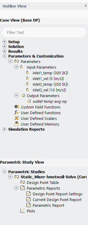
Review the elements of the initial parametric study.
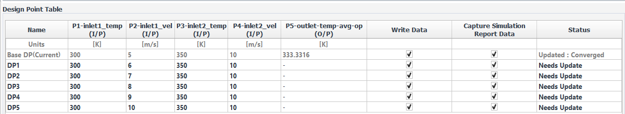
1. The Parametric Study tab that appears contains the Design Point Table with the currently loaded case file (the "base case") with its input and output parameters.
  Figure 9.3: The Design Point Table for the Initial Static Mixer Case
2. The Outline View now contains a Case View with a case-specific outline, along with a Parametric Study View that contains access to the details of your case parameters.
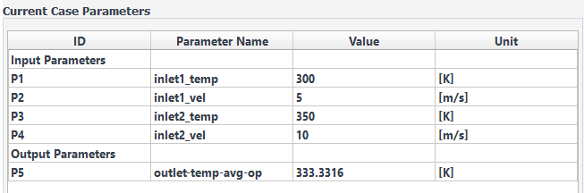
  Figure 9.4: The Case View and Parametric Study View for the Initial Static Mixer Case
3. Review details of the current case. To see the current parametric settings for the case, enable the Show Current Case Parameters option under Parametric Study in the Preferences dialog (File > Preferences...):
  Figure 9.5: The Current Parameters for the Static Mixer Case
  
  Here you can review the input and output parameters and their values and units.

9.4.4. Add Design Points

Having reviewed the parametric layout within Fluent, you can now add design points to your parametric study. For this tutorial, you will only vary the velocity at one of the two inlets, gradually increasing the value to match the velocity at the other inlet. You will also use the design point table to set various properties for each design point, such if the solution data is written, or if any simulation report-specific data is saved.

Figure 9.6: The Design Point Table With Additional Design Points

Use the Parametric ribbon to add design points to your parametric study.
Parametric → Design Point → Add Design Point
Fluent will prompt you to ensure that you want to proceed, informing you that by adding a design point, the state of the project will change (in case you wanted to preserve the current state of the project). For this tutorial, you can click Continue Adding Design Point.
In a similar fashion, add four more design points until you have a total of six, including the base design point (Base DP).
For each design point, make the following changes:
Table 9.1: Design Point Settings for the Mixing Tank
Design Point P2-inlet1_vel Enable Write Data?
DP1 6 m/s yes
DP2 7 m/s yes
DP3 8 m/s yes
DP4 9 m/s yes
DP5 10 m/s yes

Design Point	P2-inlet1_vel	Enable Write Data?
DP1	6 m/s	yes
DP2	7 m/s	yes
DP3	8 m/s	yes
DP4	9 m/s	yes
DP5	10 m/s	yes

When you later update these design points, Fluent will run each simulation using these settings and you will then be able to review their solutions and compare the results of each simulation.

9.4.5. Set Up Design Point and Parametric Reports

As described in Performing Parametric Studies, Fluent can create simulation reports for your CFD analysis. In a similar fashion, each design point run can have their own individual simulation report, as well as an overall parametric report.

Note: For this tutorial, you are not making any changes to the settings and organization of the reports. If you were to make changes to how your reports are organized, however, it is a good idea to review and change these settings as needed prior to updating the design points in your parametric study.

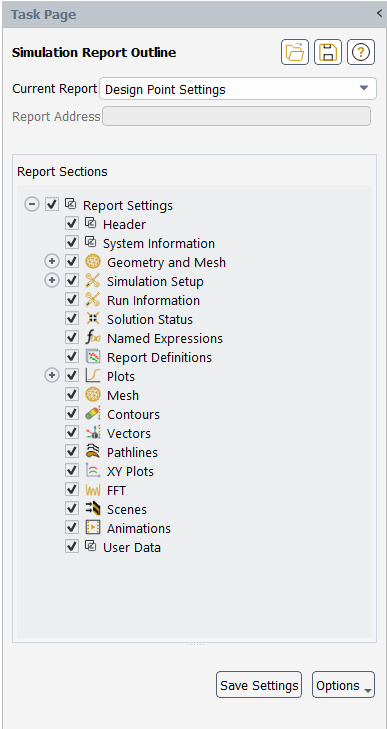
Review the settings for the individual design point simulation reports that Fluent will create.
Parametric → Simulation Report → Design Point Report Settings
This opens the Simulation Report Outline task page. When the Current Report is set to Design Point Settings, you can choose to include or exclude various portions of a typical simulation report using the Report Sections tree.
Figure 9.7: The Simulation Report Outline Task Page for Design Point Settings

For the purposes of this tutorial, you can keep the default settings.
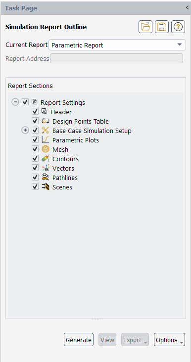
Review the settings for the overall parametric report.
When the Current Report is set to Parametric Report, you can choose to include or exclude various portions of a typical simulation report using the Report Sections tree.
Parametric → Simulation Report → Parametric Report
Figure 9.8: The Simulation Report Outline Task Page for Parameter Report Settings

For the purposes of this tutorial, you can keep the default settings.

For any given design point in the design point table, when the Capture Simulation Report Data field is enabled, the information flagged in the Simulation Report Outline for that design point will appear in the report.

9.4.6. Update Design Point Solutions

Now that the design points have been specified and the report settings have been reviewed, you can proceed to running the individual solutions and updating your design points. For this tutorial, you will use the default behavior and update each design point sequentially where each design point is loaded and solved one after another. You will also see how you can monitor the status of your various solutions as they progress.

Update all of the design points in your study.
Parametric → Update Options → Update All
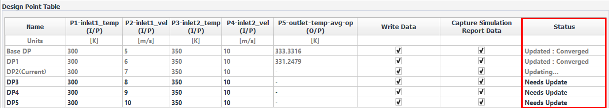
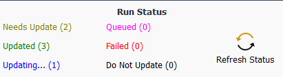
As the calculations for each design point progresses, information is printed to the console and the Status column in the Design Point Table updates accordingly.
Figure 9.9: The Status Column in the Design Point Table

You can also check the progress of your solution runs using the Run Status section of the Parametric ribbon.
Figure 9.10: The Run Status Category of the Parametric Ribbon
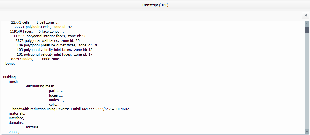
Monitor the progress of the calculation by viewing its transcript, residual plots, and plots of any solution monitors that may exist.
1. View a transcript of a design point solution by right-clicking on the design point in the table and selecting Show > Transcript from the context menu. The transcript will appear below the design point table.
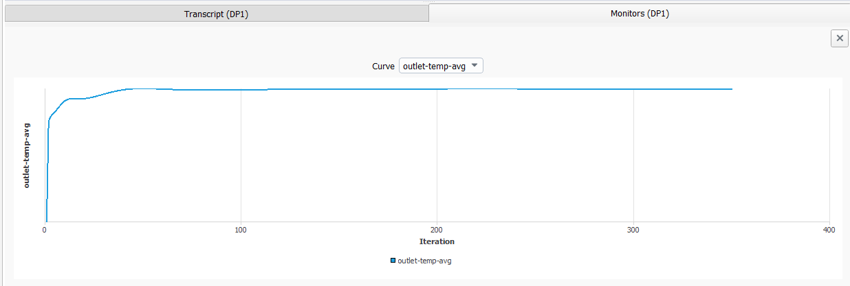
  Figure 9.11: The Transcript Window for DP1
2. View a plot of any existing solution monitors by right-clicking on the design point in the table and selecting Show > Monitors from the context menu. The monitor plot will appear below the design point table. For this tutorial, the original case file already contains a solution monitor definition (one for monitoring the average temperature at the outlet).
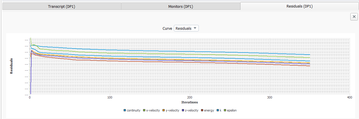
  Figure 9.12: The Monitors Window for DP1
3. View a plot of default residuals of a design point solution by right-clicking on the design point in the table and selecting Show > Residuals from the context menu. The residual plot will appear below the design point table.
  Figure 9.13: The Residuals Window for DP1

9.4.7. Generate Design Point and Parametric Simulation Reports

Now that your design points are up-to-date in your parametric study, you can create and review simulation reports for any or all of your design points.

Return to the Simulation Report Outline task page to generate an individual simulation report for one or more design points.
Parametric → Simulation Report → Design Point Report Settings
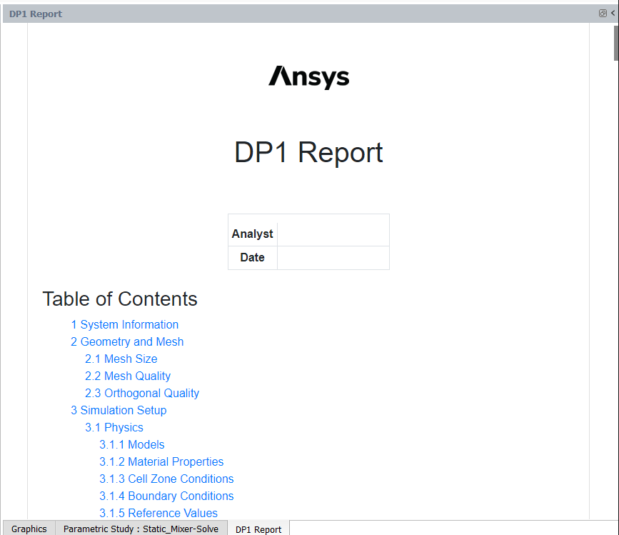
Set the Current Report to DP1 Report and click Generate at the bottom of the task page.
Once generated, the report will be displayed in the Fluent interface, tabbed alongside the graphics window.
Figure 9.14: Simulation Report for a Design Point (DP1)

You can perform the same operation for the other design points in the study (DP2 and DP3 for instance, and even the Base DP).
Based on the default selections of what the report is comprised of, the report will have tabulated information about a particular design point simulation settings. In addition, the report can include plots and animations of the mesh, contours, vectors, and pathlines of common flow field quantities (such as temperature, for instance).
Return to the Simulation Report Outline task page to generate an overall parametric report.
Parametric → Simulation Report → Parametric Report
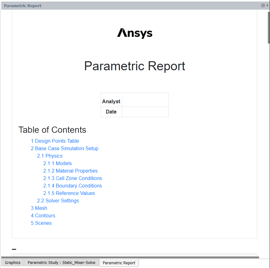
Set the Current Report to Parametric Report and click Generate at the bottom of the task page.
Once generated, the report will be displayed in the Fluent interface, tabbed alongside the graphics window.
Figure 9.15: Parametric Report

Based on the default selections of what the report is comprised of, the report will have tabulated information about the design points and the base case simulation settings. In addition, the report can include plots of the mesh, contours, vectors, and pathlines of common flow field quantities (such as temperature, for instance).

9.4.8. Compare Design Point Results

Now that you have results for all design points, you can compare the results as part of your parametric analysis. You can do this using the Parametric Report or by using Comparison Plots.

Use parametric reports to compare your results.
1. Return to the Simulation Report Outline task page to review the overall parametric report.
  Parametric → Simulation Report → Parametric Report
  Set the Current Report to Parametric Report and click View at the bottom of the task page.
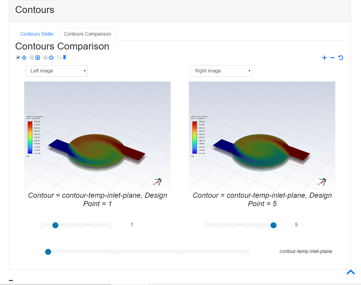
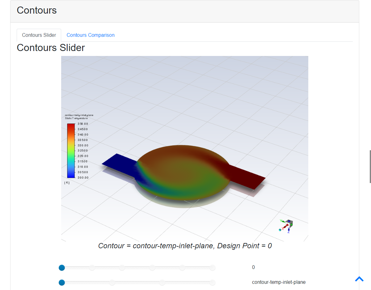
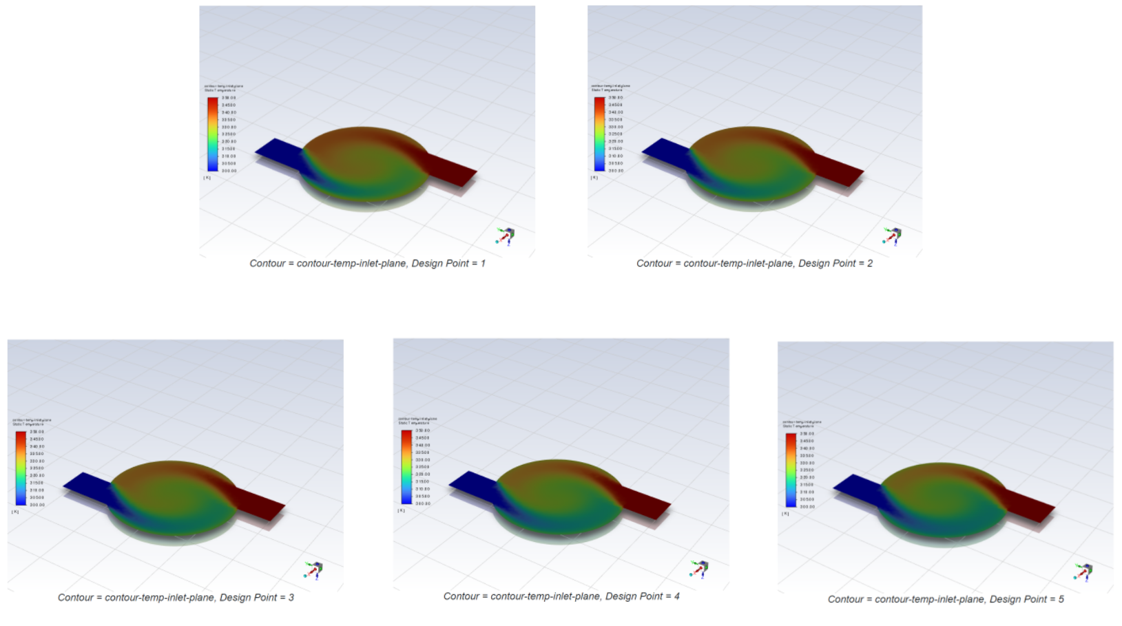
2. In the Parametric Report, go to the Contours section and review the Contours of Static Temperature plot that has been generated and included in the report.
  Figure 9.16: Contours Section of the Parametric Report (DP=0)
3. Use the slider to see the contour plot for the different design points in your study.
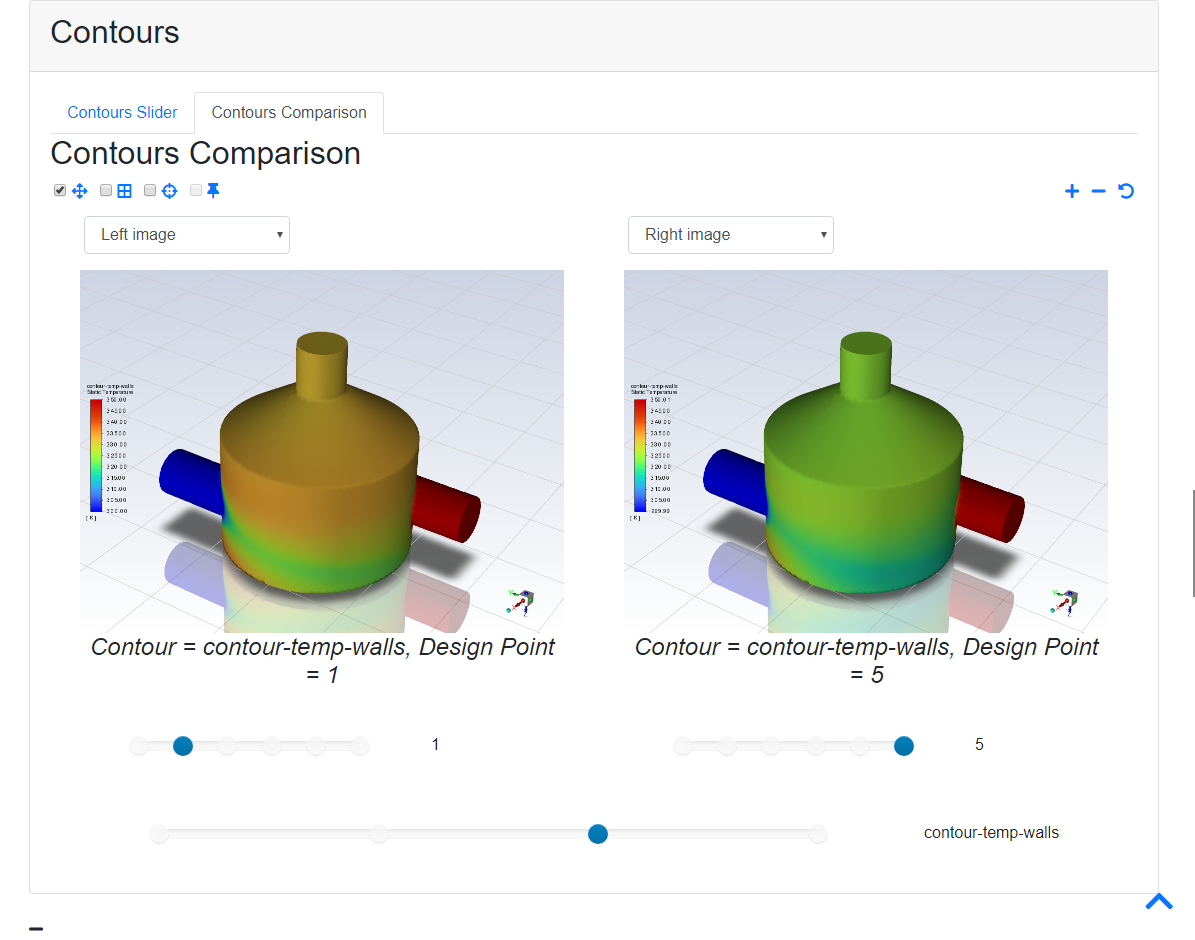
  Figure 9.17: Contours Section of the Parametric Report (All Design Points)
4. Click the Contours Comparison tab to view two plots side-by-side to compare them between two different design point values.
  Figure 9.18: Contours Section of the Parametric Report (Contour Comparison of Temperatures on the Inlet Plane)
  
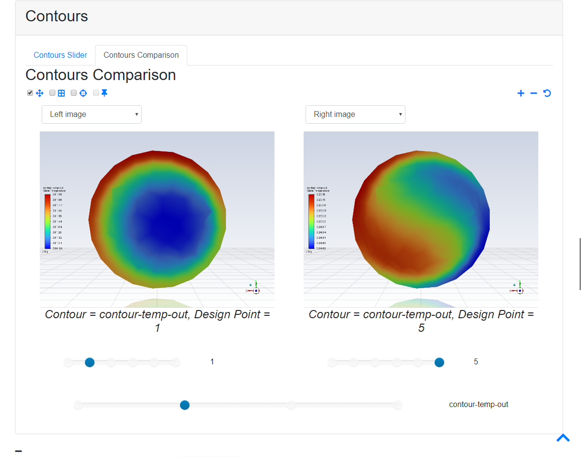
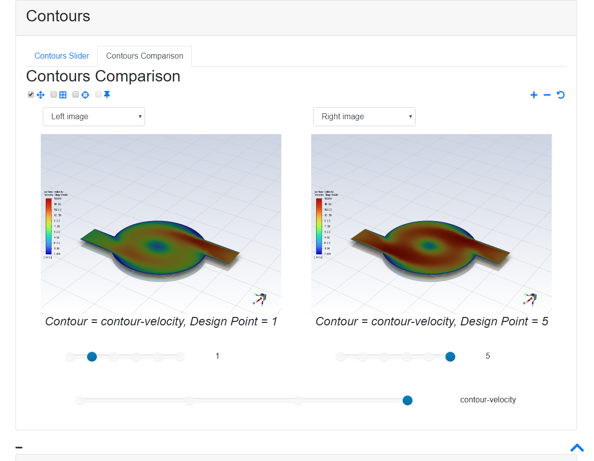
  Since there are multiple contour plots availble in the original analysis, they are also available for each design point as well. Click the bottom slider to view other available contour plot comparisons between different design points. For instance
  Figure 9.19: Contours Section of the Parametric Report (Contour Comparison of Temperature at the Outlet)
  
  Figure 9.20: Contours Section of the Parametric Report (Contour Comparison of Wall Temperature)
  
  Figure 9.21: Contours Section of the Parametric Report (Contour Comparison of Velocity)
  
  For more information about comparing plots in your simulation reports, see Comparing Parametric Results.
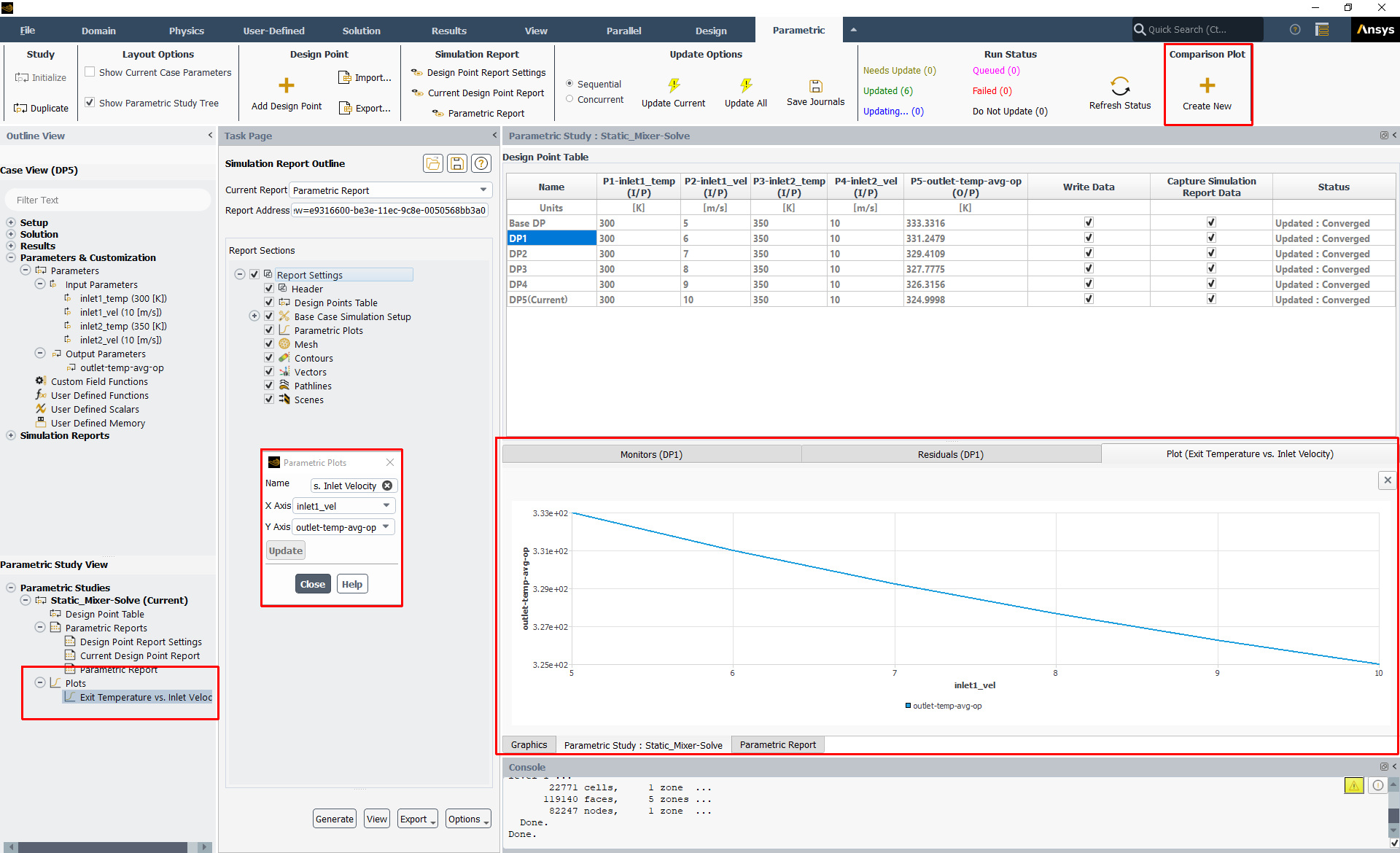
Use comparison plots to compare the input and/or output parameter values as they vary with each other or by design point.
Parametric → Comparison Plot → Create New
This opens the Parametric Plots dialog box where you can specify the details of a comparison plot.
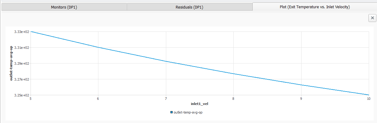
1. For the Name, enter Exit Temperature vs Inlet Velocity.
2. For the X Axis, select inlet1_vel.
3. For the Y Axis, select outlet-temp-avg-op.
4. Click Create to visualize the plot under the Design Point Table. A new plot is created in the Parametric Study View under Plots.
5. Close the dialog box.
Figure 9.22: Elements of Comparison Plots

Figure 9.23: Plot of Exit Temperature vs Inlet Velocity Value
Save the case and data files (Static_Mixer.cas.h5 and Static_Mixer.dat.h5).
File → Write → Case & Data...
Save the project file (Static_Mixer.flprj).
File → Parametric Project → Save...

9.5. Summary

This tutorial demonstrated taking an existing singular Fluent case and data file set with input and output parameters and developing a parametric study directly in the Ansys Fluent interface. Variations of those input parameters were used to create different solutions for comparative analysis. Individual design points were analyzed and simulation reports were generated for each design point and for the parametric study itself. Finally, simulation reports and comparative plots were used to examine the changes of an input variable per design point. For more information about using Fluent to perform a parametric analysis, refer to Performing Parametric Studies.