Chapter 10: Optimizing Parametric Analyses in Ansys Fluent

This tutorial is divided into the following sections:

10.1. Introduction

This tutorial illustrates how to perform an optimized parametric analysis of a two-dimensional flow simulation within Ansys Fluent using Ansys optiSLang. The analysis will take an existing Fluent case file with predefined input and output parameters, and setup and solve various permutations that analyze a few changes to the parametric variables, all within the Fluent interface. For more information about using Fluent to perform an optimized parametric analysis, refer to Performing Parametric Studies.

Note: An Ansys optiSLang license is requried for this tutorial.

Note: Ansys optiSLang provides several ways to perform parametric optimizations, including One-Click Optimization (OCO) and the more powerful Adaptive Metamodel of Optimal Prognosis (AMOP) approach. For the sake of simplicity, this tutorial focuses on the OCO approach to optimization. For more information, see Creating and Optimizing Designs of Experiments for optiSLang.

This tutorial demonstrates how to do the following:

Start with a Fluent case and data file with input and output parameters.
Apply mesh morphing to define changes in the geometry and the mesh using input parameters.
Use One-Click Optimization (OCO) and Ansys optiSLang within Fluent to define and generate a series of additional cases (design points) where each represents a change to one or more of the parameters.
Generate a simulation report for each design point.
Review the simulation reports and perform a comparison of the results between design points.

Related video that demonstrates steps for setting up, solving, and postprocessing a parametric study in Fluent:

10.2. Prerequisites

This tutorial is written with the assumption that you have completed one or more of the introductory tutorials (such as Fluid Flow and Heat Transfer in a Mixing Elbow) found in this manual and that you are familiar with the Ansys Fluent tree and ribbon structure. Some steps in the setup and solution procedure will not be shown explicitly.

10.3. Problem Description

The problem being analyzed involves a two dimensional heat exchanger geometry with an inlet and an outlet.

Figure 10.1: Problem Schematic

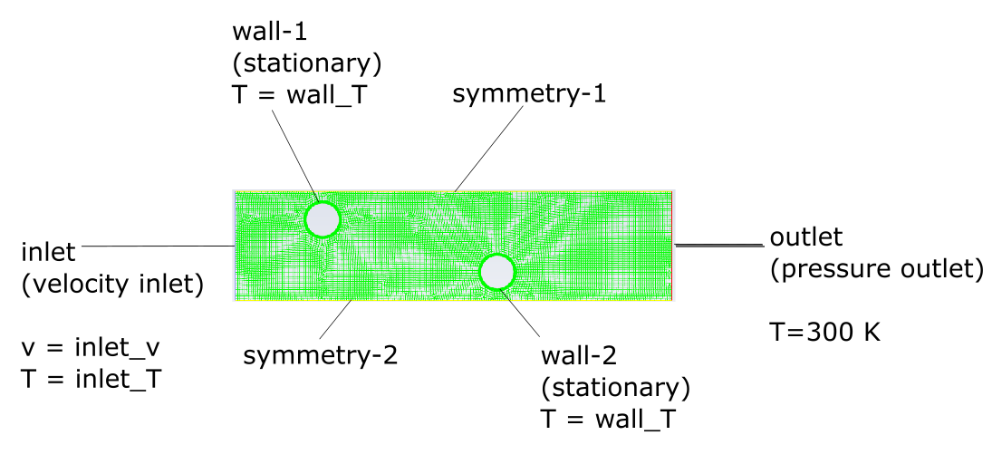
Fluid enters a two-dimensional heat exchanger through a single inlet using conditions described by separate input parameter expressions for the fluid velocity magnitude (inlet_v) and temperature (inlet_T). The fluid exits the outlet of the heat exchanger based on a pressure outlet condition with a temperature of 300 Kelvin. The parametric analysis will study the best displacement of the cylinders while studying the heat transfer and optimizing the pressure drop across the heat exchanger.

The input parameter expressions are initially set to the following constant values:

Input Parameter	Value
`inlet_T`	300 K
`inlet_v`	2.5 m/s
`wall_1_dx`	0 m
`wall_1_dy`	0 m
`wall_2_dx`	0 m
`wall_2_dy`	0 m

The following named expressions are defined as:

Named Expression	Value
`flow_energy`	`{report-av-inlet-pressure}*{report-mass-flow-rate}/1.225[kg/m^3]`
`heat_transfer_per_flow_energy`	`{total_heat_transfer}/flow_energy`
`wall_T`	500 K

The output parameters are defined accordingly:

Ouput Parameter	Value
`heat_transfer_per_flow_energy`	`{total_heat_transfer}/flow_energy`
`min-orth-quality-op_v`	Volume report defintion of the minimal mesh orthogonal quality for the fluid zone.
`report-fx-1-op`	Force report defintion for the first wall.
`report-fx-2-op`	Force report defintion for the second wall.
`report-out-press-op`	Surface report defintion for the area-weighted average of the staic pressure at the inlet.
`report-out-temp-op`	Surface report defintion for the mass-weighted average of the static temperature at the outlet.
`total_heat_transfer`	Flux report definition for the total hat transfer rate for the circular walls.

Note: The OCO approach to optimization only allows you to have a single objective. Therefore, a combined output parameter was defined to represent both the heat transfer and the pressure drop. The objective defined allows you to maximize the combined output paramater.

10.4. Setup and Solution

The following sections describe the setup and solution steps for this tutorial:

10.4.1. Preparation

To prepare for running this tutorial:

Download the 2d_heat_exchanger_optimizer.zip file here .
Unzip 2d_heat_exchanger_optimizer.zip to your working directory.
The files 2d_heat_exchanger.cas.h5 and 2d_heat_exchanger.dat.h5 can be found in the folder.
Use the Fluent Launcher to start Ansys Fluent.
Select Solution in the top-left selection list to start Fluent in Solution Mode.
Select 2D under Dimension.
Enable Double Precision under Options.
Set Solver Processes to 4 under Parallel (Local Machine).

10.4.2. Mesh

Read the case and data file (2d_heat_exchanger.cas.h5 and 2d_heat_exchanger.dat.h5).
File → Read → Case & Data...
As Fluent reads the case/data files, it will report the progress in the console.
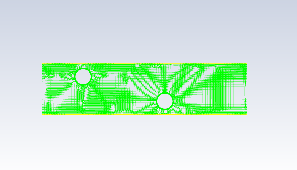
Examine the mesh (Figure 10.2: Mesh Display of the 2D Heat Exchanger Geometry).
Note: You can use the right mouse button to check which zone number corresponds to each boundary. If you click the right mouse button on one of the boundaries in the graphics window, its zone number, name, and type will be printed in the Ansys Fluent console. This feature is especially useful when you have several zones of the same type and you want to distinguish between them quickly.
Figure 10.2: Mesh Display of the 2D Heat Exchanger Geometry

10.4.3. Applying Mesh Morphing

For this particular tutorial, the parametric optimization is designed to determine the best location of the circular walls in the heat exchanger under specific conditions. Such an analysis requires changes to the geometry/mesh for each parametric design point. You can perform such changes in the geometry/mesh directly in Fluent through the use of mesh morphing.

Note: The following steps have been applied upon loading the case file. However, this section is for demonstrative purposes to reveal what those steps were.

Define your design conditions.
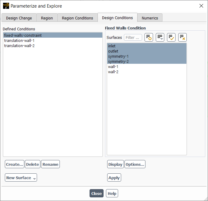
Design → Geometry → Parameterize and Explore
1. Create a fixed wall constraint condition to be applied to the inlet, outlet and the symmetry boundaries.
  Figure 10.3: Setting Fixed Wall Constraint Conditions
  1. In the Parameterize and Explore dialog box, in the Design Conditions tab, click Create... to display the Create New Condition dialog box.
  2. In the Create New Condition dialog box, select fixed-walls-constraint and change the Name to fixed-walls-constraint.
  3. Click OK to create the new condition and close the Create New Condition dialog box.
  4. In the Parameterize and Explore dialog box, in the Design Conditions tab, for the new fixed-walls-constraint condition, under Fixed Walls Condition, select the inlet, outlet, symmetry-1, and symmetry-2 surfaces and click Apply.
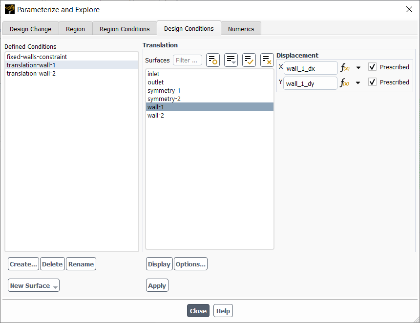
2. Create a translating wall condition to be applied to one of the circular walls.
  Figure 10.4: Setting Translating Wall Conditions (wall-1)
  1. In the Parameterize and Explore dialog box, under Design Conditions, click Create... to display the Create New Condition dialog box.
  2. In the Create New Condition dialog box, select translation and change the Name to translation-wall-1.
  3. Click OK to create the new condition and close the Create New Condition dialog box.
  4. In the Parameterize and Explore dialog box, for the new translation-wall-1 condition, under Fixed Walls Condition, select the wall-1 surface.
  5. Assign the wall_1_dx named expression for the X displacement.
  6. Assign the wall_1_dy named expression for the Y displacement.
  7. Click Apply.
3. Create a second translating wall condition to be applied to the other circular wall.
  Figure 10.5: Setting Translating Wall Conditions (wall-2)
  1. In the Parameterize and Explore dialog box, under Design Conditions, click Create... to display the Create New Condition dialog box.
  2. In the Create New Condition dialog box, select translation and change the Name to translation-wall-2.
  3. Click OK to create the new condition and close the Create New Condition dialog box.
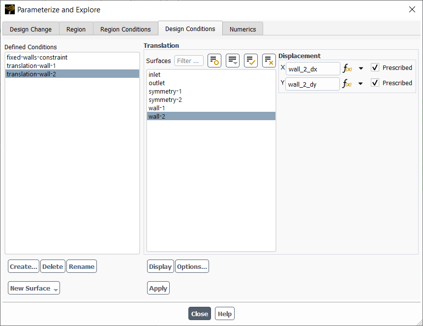
  4. In the Parameterize and Explore dialog box, for the new translation-wall-2 condition, under Fixed Walls Condition, select the wall-2 surface.
  5. Assign the wall_2_dx named expression for the X displacement.
  6. Assign the wall_2_dy named expression for the Y displacement.
  7. Click Apply.
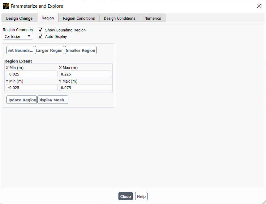
Define your design region.
Figure 10.6: The Region Tab of the Parameterize and Explore Dialog Box

In the Parameterize and Explore dialog box, in the Region tab, under Region Extent, set the following values:
X Min -0.025 m
X Max 0.225 m
Y Min -0.025 m
Y Max 0.075 m
Check and preview the mesh morphing settings.
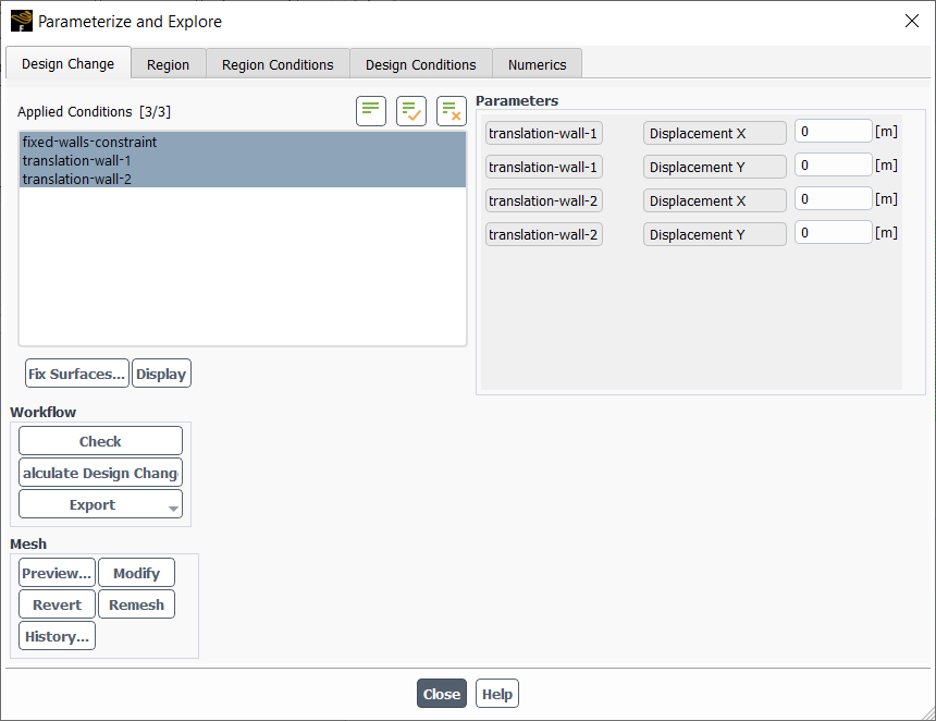
Figure 10.7: The Design Change Tab of the Parameterize and Explore Dialog Box
1. In the Parameterize and Explore dialog box, in the Design Change tab, review your settings and, under Workflows, click Check to confirm your settings.
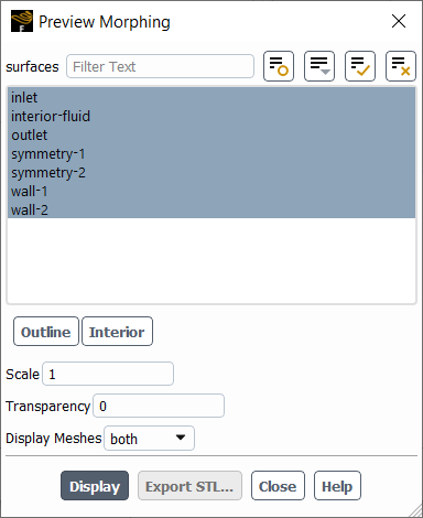
2. Once your settings are confirmed, under Mesh, click Preview... to visually inspect the mesh morphing region extents using the Preview Morphing dialog box.
  Figure 10.8: Preview Morphing Dialog Box
  
  In the Preview Morphing dialog box, select all surfaces and click Display.
  Figure 10.9: Preview of the Mesh Morphing Region

Now that parameter-based changes in the mesh are accounted for through setting up mesh morphing, you can proceed on to setting up and optimizing the parametric study.

10.4.4. Initialize the Parametric Study

Using your loaded case file with predefined input parameters, you can start the parametric study.

Initialize the parametric study.
Parametric → Study → Initialize
Create a project file (2d_heat_exchanger.flprj).
You will need to manage various files that get created for your parametric study, so Fluent will prompt you to create a new project file to help manage the files that will be generated for each design point run. Click Yes to proceed with creating a project file. Fluent will prompt you for the name and location of the project file. For this tutorial, keep the default name as 2d_heat_exchanger.flprj and keep the location as your current working folder.
Note: Once you create a project file, you can revisit it at any time by opening the project file using the File menu.
File → Parametric Project → Open...
Review the elements of the initial parametric study.
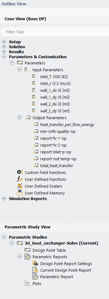
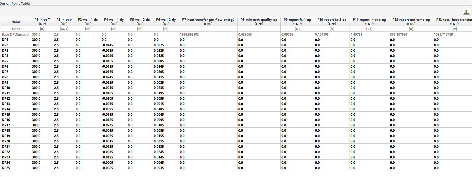
1. The Parametric Study tab that appears contains the Design Point Table with the currently loaded case file (the "base case") with its input and output parameters.
  Figure 10.10: The Design Point Table for the Initial 2D Heat Exchanger Case
2. The Outline View now contains a Case View with a case-specific outline, along with a Parametric Study View that contains access to the details of your case parameters.
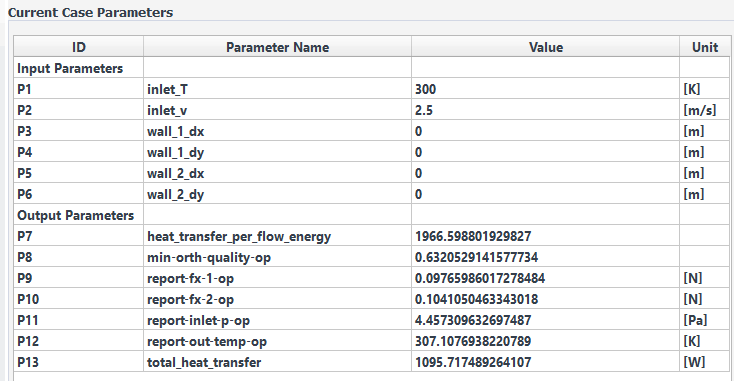
  Figure 10.11: The Case View and Parametric Study View for the Initial 2D Heat Exchanger Case
3. Review details of the current case. To see the current parametric settings for the case, enable the Show Current Case Parameters option under Parametric Study in the Preferences dialog (File > Preferences...):
  Figure 10.12: The Current Parameters for the 2D Heat Exchanger Case
  
  Here you can review the input and output parameters and their values and units.

10.4.5. Set Up Design Point and Parametric Reports

As described in Performing Parametric Studies, Fluent can create simulation reports for your CFD analysis. In a similar fashion, each design point run can have their own individual simulation report, as well as an overall parametric report.

Note: For this tutorial, you are not making any changes to the settings and organization of the reports. If you were to make changes to how your reports are organized, however, it is a good idea to review and change these settings as needed prior to updating the design points in your parametric study.

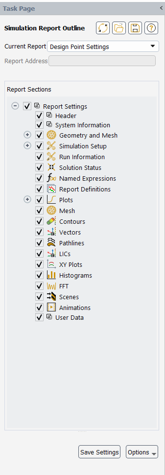
Review the settings for the individual design point simulation reports that Fluent will create.
Parametric → Simulation Report → Design Point Report Settings
This opens the Simulation Report Outline task page. When the Current Report is set to Design Point Settings, you can choose to include or exclude various portions of a typical simulation report using the Report Sections tree.
Figure 10.13: The Simulation Report Outline Task Page for Design Point Settings

For the purposes of this tutorial, you can keep the default settings.
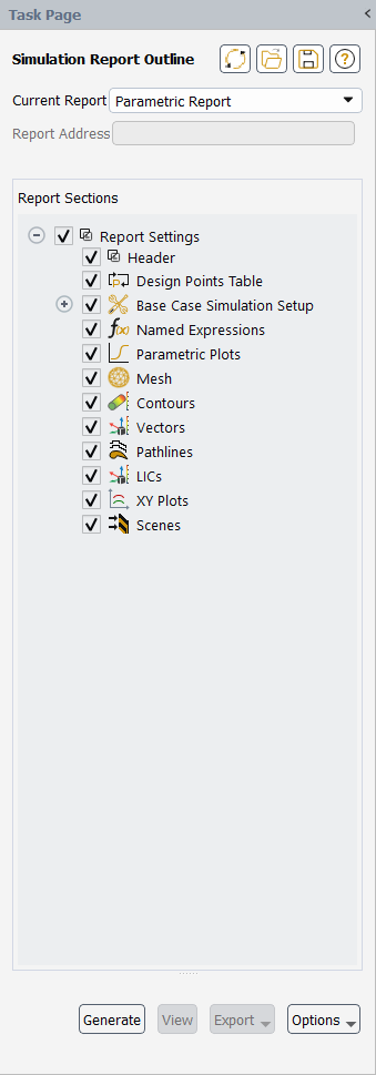
Review the settings for the overall parametric report.
When the Current Report is set to Parametric Report, you can choose to include or exclude various portions of a typical simulation report using the Report Sections tree.
Parametric → Simulation Report → Parametric Report
Figure 10.14: The Simulation Report Outline Task Page for Parameter Report Settings

For the purposes of this tutorial, you can keep the default settings.

For any given design point in the design point table, when the Capture Simulation Report Data field is enabled, the information flagged in the Simulation Report Outline for that design point will appear in the report.

10.4.6. Create Design Points and Run an Optimization Study

Having reviewed the parametric layout within Fluent, you can now add design points to your parametric study. For this tutorial, you will use the built-in optimization tools in Fluent to define a series of design points.

Parametric → Design Point → Auto (with optiSLang) → Add Design Points...

This displays the Create Design Points Using optiSLang dialog box. Select the Create DOE and Optimize option to display more options in the Create Design Points and Optimize Using optiSLang dialog box.

Figure 10.15: The Create Design Points and Optimize Using optiSLang Dialog Box

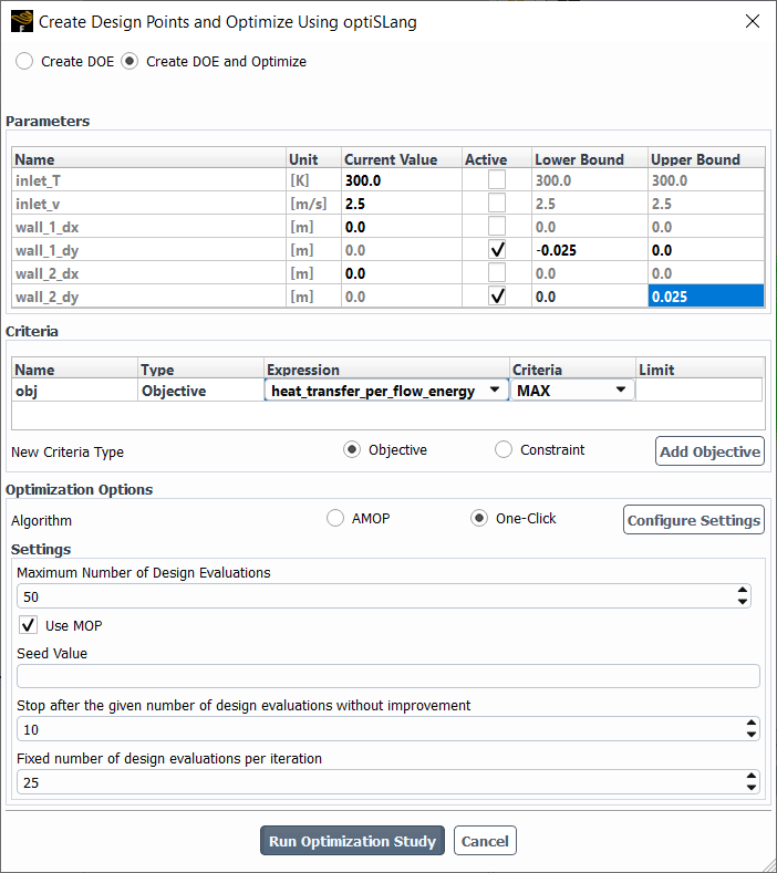
Edit the parameters.
1. De-activate the inlet_T, inlet_v, wall_1_dx, and wall_2_dx parameters in the table.
2. Set the Lower Bound for wall_1_dy to -0.025.
3. Set the Upper Bound for wall_2_dy to 0.025.
Edit the criteria.
Under Criteria, keep the New Criteria Type set to Objective, and click Add Objective to display a new objective criteria. For the new criteria:
1. Set the Expression to heat_transfer_per_flow_energy.
  The OCO approach to optimization only allows you to have a single objective. Therefore, a combined output parameter was defined to represent both the heat transfer and the pressure drop. The objective defined allows you to maximize the combined output paramater.
2. Set the Criteria to MAX.
Edit the one-click optimization (OCO) settings.
Under Optimization Options, select One-Click and click Configure Settings to directly expose additional optiSLang settings.
1. Set the Maximum Number of Design Evaluations to 50.
  Once this field is set, a brief pause may occur as optiSLang updates the remaining fields.
2. Ensure that the Stop after the given number of design evaluations without improvement option is to 10.
3. Ensure that the Fixed number of design evaluations per iteration option is set to 25.
Click Run Optimization Study.
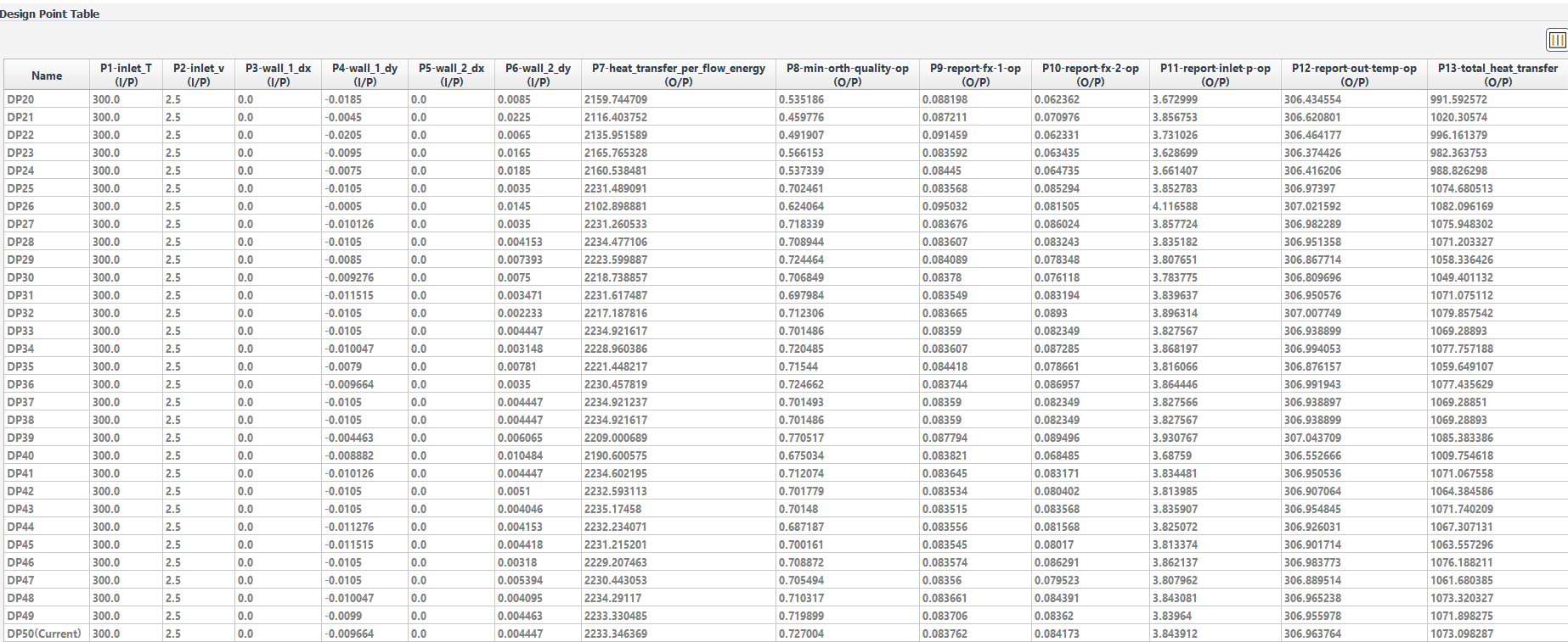
Fluent will automatically run each design point simulation using these settings, generate data, and update the design point table accordingly.
Figure 10.16: The Design Point Table With Initial Optimization Study Design Point Data

Once the optimization study is complete, you will then be able to review their solutions and compare the results of each simulation.
Figure 10.17: The Design Point Table With Final Optimization Study Design Point Data

Click the Show Optimization Results button to display the tabulated display of the one-click optimization study.
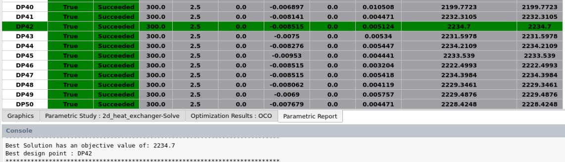
Figure 10.18: The Results of the Optimization Study Showing the Best Solution

10.4.7. Generate Design Point and Parametric Simulation Reports

Now that your design points are up-to-date in your parametric study, you can create and review simulation reports for any or all of your design points. For this tutorial, you will generate a design point report for the solution that was identified as the optimal solution (DP42).

Return to the Simulation Report Outline task page to generate an individual simulation report for one or more design points.
Parametric → Simulation Report → Design Point Report Settings
Set the Current Report to DP42 Report and click Generate at the bottom of the task page.
Once generated, the report will be displayed in the Fluent interface, tabbed alongside the graphics window.
Figure 10.19: Simulation Report for the Optimal Design Point (DP42)

Based on the default selections of what the report is comprised of, the report will have tabulated information about a particular design point simulation settings. In addition, the report can include plots and animations of the mesh, contours, vectors, and pathlines of common flow field quantities (such as temperature, for instance).
Return to the Simulation Report Outline task page to generate an overall parametric report.
Parametric → Simulation Report → Parametric Report
Set the Current Report to Parametric Report and click Generate at the bottom of the task page.
Once generated, the report will be displayed in the Fluent interface, tabbed alongside the graphics window.
Figure 10.20: Parametric Report

Based on the default selections of what the report is comprised of, the report will have tabulated information about the design points and the base case simulation settings. In addition, the report can include plots of the mesh, contours, vectors, and pathlines of common flow field quantities (such as temperature, for instance).

10.4.8. Compare Design Point Results

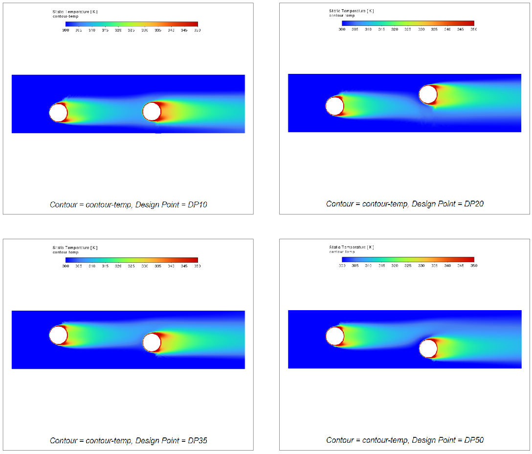
Now that you have results for all design points, you can compare the results as part of your parametric analysis. You can do this using the Parametric Report or by using Comparison Plots.

Use parametric reports to compare your results.
1. Return to the Simulation Report Outline task page to review the overall parametric report.
  Parametric → Simulation Report → Parametric Report
  Set the Current Report to Parametric Report and click View at the bottom of the task page.
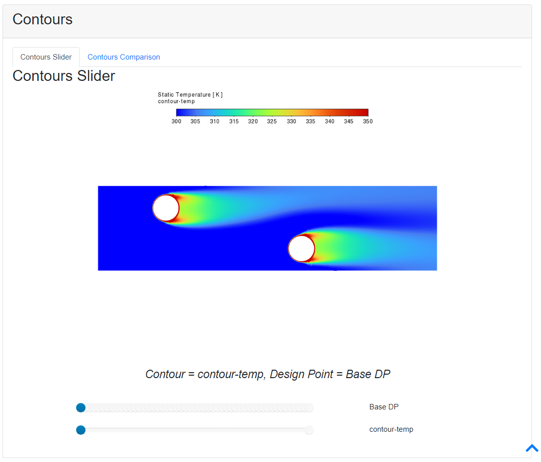
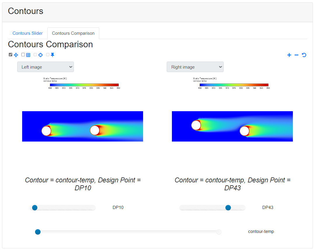
2. In the Parametric Report, go to the Contours section and review the Contours of Static Temperature plot that has been generated and included in the report.
  Figure 10.21: Contours Section of the Parametric Report (DP=0)
3. Use the slider to see the contour plot for the different design points in your study.
  Figure 10.22: Contours Section of the Parametric Report (Select Design Points)
4. Click the Contours Comparison tab to view two plots side-by-side to compare them between two different design point values.
  Figure 10.23: Contours Section of the Parametric Report (Contour Comparison of Temperatures)
  
  For more information about comparing plots in your simulation reports, see Comparing Parametric Results.
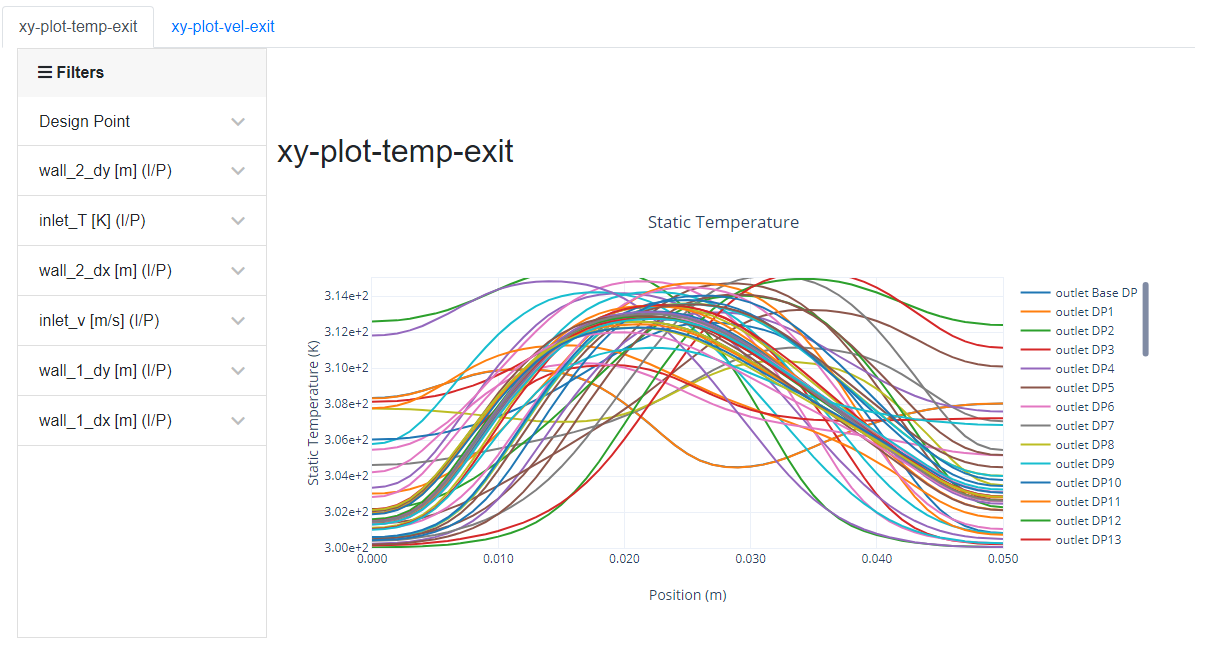
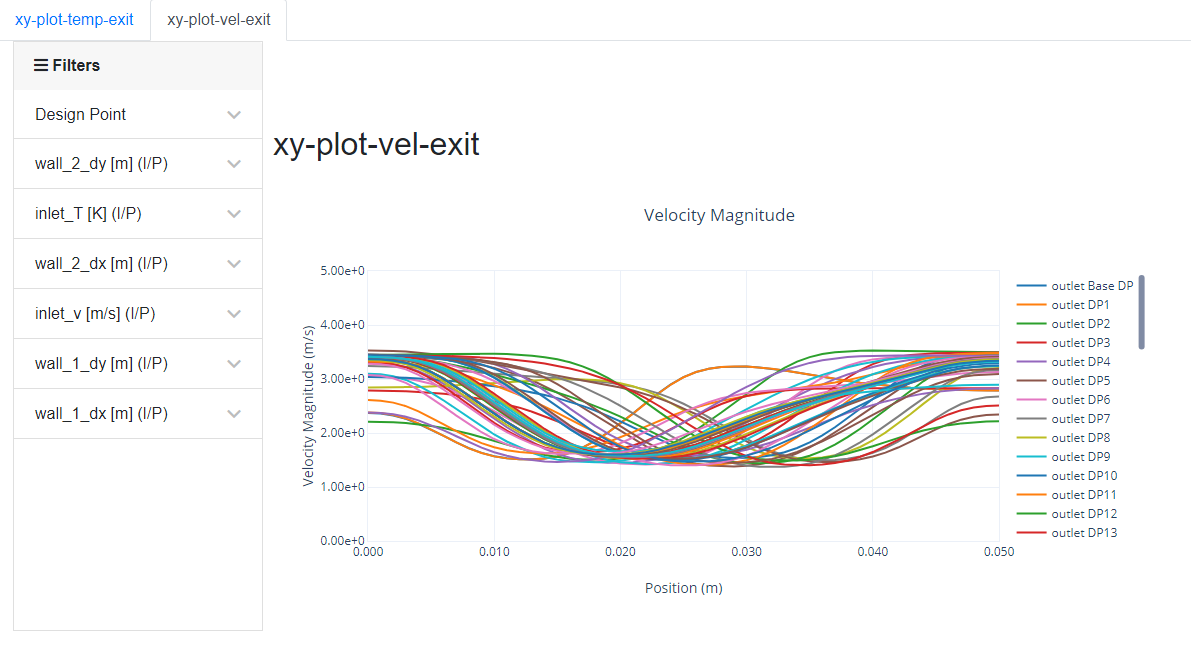
5. In the Parametric Report, go to the XY Plots section and review the static temperature (xy-plot-temp-exit) and the velocity magnitude (xy-plot-vel-exit) plots that have been generated and included in the report.
  Figure 10.24: Static Temperature Distribution at the Exit for All Design Points
6. Figure 10.25: Velocity Magnitude Distribution at the Exit for All Design Points
Save the case and data files (2d_heat_exchanger.cas.h5 and 2d_heat_exchanger.dat.h5).
File → Write → Case & Data...
Save the project file (2d_heat_exchanger.flprj).
File → Parametric Project → Save...

10.5. Summary

This tutorial demonstrated taking an existing singular Fluent case and data file set with input and output parameters and developing a optimization parametric study directly in the Ansys Fluent interface using Ansys optiSLang. Since the parametric analysis involved geometry/mesh changes, Fluent's mesh morphing capabilities were utilized. Fluent was used to easily set up a one-click optimization study where variations of those input parameters were used to create different solutions for comparative analysis. Individual design points were analyzed and simulation reports were generated for each design point and for the parametric study itself. Finally, simulation reports were used to examine the changes of an input variable per design point. For more information about using Fluent to perform a parametric analysis, refer to Performing Parametric Studies.

X Min	`-0.025` m
X Max	`0.225` m
Y Min	`-0.025` m
Y Max	`0.075` m