The following sections of this chapter are:
This tutorial explains how to optimize the design of a bleed-air (piccolo tube) anti-icing system located inside the protected zone of a wing’s leading edge using a dedicated Ansys Workbench utility called IPSOPT. You will learn how to set up, monitor and post-process a single-objective optimization scenario with multiple constraints and design variables, while using a set of in-flight icing conditions called a condition matrix. The optimization of a piccolo tube design is a multidisciplinary problem that involves not only the IPSOPT system and its components, but also other applications such as ICE3D and DesignXplorer to complete the optimization cycle.
The following briefly describes the set-up of a piccolo tube design optimization cycle in Ansys Workbench:
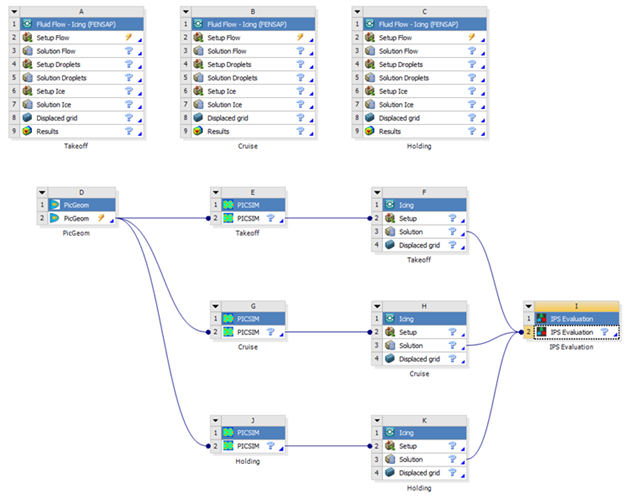
Start by setting up PicGeom to define the design variables and geometric parameters of the piccolo tube and connect this component to PICSIM.
For each in-flight icing condition, PICSIM solves the flow inside the piccolo tube based on a 1D pipe flow model and generates internal Heat Transfer Coefficients (HTCs) on the inner skin of the protected zone. These HTCs represent the heating pattern and intensity provided by the hot-air jets produced by the orifices of the piccolo tube that are expected to prevent ice formation on the protected zone. Each Workbench component is then connected to a single ICE3D module.
ICE3D computes the thermal balance between the in-flight icing condition and the corresponding internal HTC distribution provided by PICSIM. All the ICE3D solutions are then linked to a single IPS Evaluation component.
IPS Evaluation finds the most critical in-flight icing condition in the condition matrix based on a user-defined set of constraints and objectives. This component is then linked to DesignXplorer.
DesignXplorer (DX) and Workbench Parameter Set capabilities will be utilized to define the optimization method, explore the design space to find the best possible design point, visualize the results of the optimization, and trace the evolution of the design space, constraints and objectives of the design optimization cycle of the piccolo tube system.
In depth description of the procedure as well as installation of the appropriate Ansys Workbench add-ons are covered in this tutorial. This tutorial therefore addresses the following processes:
Launch Ansys Workbench.
Install the IPSOPT Add-on.
Create an IPSOPT system components in Ansys Workbench for a flight condition matrix.
Set up the geometric parameters and design variables of the piccolo tube inside PicGeom.
Set up the piccolo tube simulation in PICSIM.
Set up the icing simulation in the Icing component.
Set up the optimization scenario in IPS Evaluation to search for the most adverse in-flight icing condition of the condition matrix.
Define the optimization method, constraints, objectives and design space in DesignXplorer.
Analyze the results and produce the optimization charts.
Commercial aircraft must be certified to Fly into Known Icing Conditions (FIKI). An unrealistic amount of power that far exceeds the power produced by the engines would be required to protect a complete aircraft against icing, hence only the critical surfaces are actively protected. Due to the constant drive to improve efficiency and reduce fleet operating costs, all aircraft systems are highly optimized, with the exception of bleed air systems up to now, due to the complexity of the icing phenomena and the lack of accurate computational tools for their simulation.
The purpose of this tutorial is to find the optimal or “best” feasible piccolo tube configuration(s) that minimize(s) the required supply of bleed air to the IPS while protecting the critical area from ice accretion and preventing water runback past the protected zone limit on the upper surface of the wing. Three in-flight icing conditions are considered in this tutorial. Thus, the optimal piccolo tube configuration(s) should prevent ice accretion and water runback past the protected zone on the upper surface of the wing for all of these conditions. A schematic of the geometric parameters and flow properties of a piccolo tube is shown in Figure 1.4: Schematic of a Piccolo Tube.
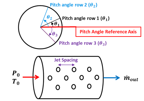
In this tutorial, only the spacing between piccolo hole centers and the pitch angles between piccolo hole rows are design variables that can change during the optimization. The number of rows, in this case three rows of piccolo holes, as well as the piccolo hole diameter, in this case 1mm, remain fixed during the design optimization of the piccolo tube.
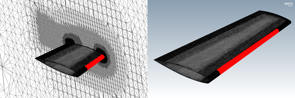
In order to prevent ice accretion over the protected area (Figure 1.5: Wing External Mesh Surface with Protected Area in Red), a minimum wall temperature higher than the freezing temperature is imposed as a design constraint. In this tutorial, the minimum allowable wall temperature is 276 K. A maximum wall temperature is also imposed as a constraint and its value is 440 K. Since the upper surface of a wing is, in general, a more critical surface to protect against icing than the lower surface, a constraint that prevents water runback past the upper surface of the protected zone is imposed. No water runback constraint is applied on the lower surface of the protected zone.
This scenario is therefore a single-objective optimization problem with 3 constraints and 4 design variables. These are listed in Table 1.1: Optimization Scenario.
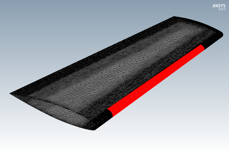
Table 1.1: Optimization Scenario
| Type | Name | Reference value |
|---|---|---|
| Objective | Minimize Piccolo Tube Mass Flow Rate | |
| Constraint | Minimum Surface Temperature | 276 K |
| Constraint | Maximum Surface Temperature | 440 K |
| Constraint | Upper Surface End Limit Film Height | 0 microns |
| Design Variable | Pitch Angle of Row 1 | |
| Design Variable | Pitch Angle of Row 2 | |
| Design Variable | Pitch Angle of Row 3 | |
| Design Variable | Center-to-center Jet Spacing |
Download the Beta_Optimization_Piccolo_Tube_Ice_Protection_System.zip file here .
Unzip Beta_Optimization_Piccolo_Tube_Ice_Protection_System.zip into your working directory. This file contains the external grid of the ONERA M6 wing in FENSAP format (../workshop_input_files/Grid/oneram6.grd).
Note: You need a basic knowledge of FENSAP-ICE and Workbench to set up these airflow and droplet simulations. If you require further training on these applications, see Introductory Tutorials to In-Flight Icing within the FENSAP-ICE Tutorial Guide.
Open Ansys Workbench.
To install the IPSOPT add-on, choose Extensions → Install Extension… and select the IPSOPT-WB.wbex file located in your installation subdirectory (../fensapice/workbench). A dialog box will appear, select OK to confirm.
To activate the IPSOPT extension, choose Extensions → Manage Extensions…. In the Extension Manager dialog, click to select the IPSOPT-WB extension. Right-click and choose Load to run once, or Load as Default to load the IPSOPT-WB extension every time you start Workbench. Close the Extension Manager.
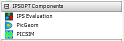
Once you have loaded the extension, you will see IPSOPT Components listed in the Workbench Toolbox as a new system. The Workbench Toolbox contains the following IPSOPT system template:
If the FENSAP-ICE add-on is not installed in your Workbench, follow these steps:
To install the FENSAP-ICE add-on, choose Extensions → Install Extension… and select the FENSAPICE-WB.wbex file located in your installation subdirectory (../fensapice/workbench). A dialog box will appear, select OK to confirm.
To activate the extension, choose Extensions → Manage Extensions…. In the Extension Manager dialog, click to select the FENSAPICE-WB extension. Right-click and choose Load to run once or Load as Default to load the FENSAPICE-WB extension every time you start Workbench. Close the Extension Manager.
The external airflow and water droplet solutions are computed for each in-flight icing condition using a Fluid Flow-Icing (FENSAP) system. These solutions are not updated during the optimization of the piccolo tube and therefore serve only as inputs to the piccolo tube optimization system.
To load these solutions and their respective systems in Workbench, go to File → Open and load the Workbench project external-airflow.wbpj located in the folder External_Flow_Droplet of your working directory. This project contains three in-flight icing solutions computed over a 3D ONERA-M6 wing.
The ONERA-M6 grid is an unstructured grid of approximately 3.5 million nodes composed of tetrahedral and prism elements to capture the boundary layer over the geometrical model. This grid is shown in Figure 1.6: ONERA M6 Wing External Mesh. The KW-SST with Intermittency turbulence model was used to capture the boundary layer and its transition from laminar to turbulent flow. The fluid domain is bound by a symmetry plane and a far-field boundary.
In this project, the three in-flight icing conditions correspond to takeoff, cruise and holding conditions. The external air flow and droplet conditions are provided in the following table:
Table 1.2: Flight and Icing Condition Matrix
| Flight Condition | Ps (Pa) | Ts (K) | V (m/s) | AOA (deg) |
MVD (µm) Monodispersed | LWC (g/m3) |
|---|---|---|---|---|---|---|
| Takeoff | 101,325 | 270 | 80 | 0 | 20 | 0.57079 |
| Cruise | 44,081.324 | 254 | 175 | 5 | 20 | 0.231329634 |
| Holding | 54,054 | 263 | 115 | 8 | 20 | 0.421875043 |
If you would like to conduct these simulations in a different Workbench project, follow the steps described in In-Flight Icing Using CFX Within Workbench in the FENSAP-ICE Tutorial Guide and replace its condition by the conditions shown in Table 1.2: Flight and Icing Condition Matrix. In addition, pay attention to the following settings:
Airflow Settings
Use the external grid (oneram6.grd) located in ../workshop_input_files/Input_Grid/Grid. You can either copy the grid in each fluid flow directory or create a link to the Grid directory.
Activate the K-omega SST turbulence model and its transition model, Intermittency.
Specify an Eddy/Laminar viscosity ratio and a Turbulence intensity of
1e-05and0.0008respectively.No sand-grain roughness should be applied on the walls of the ONERA-M6.
Select Supersonic or far-field for the Inlet conditions and Adiabatic Stagn. temp. + 10 (all walls) for the all Wall conditions.
Decrease the Cross-wind dissipation to
1e-09and the Convergence level to1e-15.Run the takeoff condition using
2000Solver iterations and a CFL number of100. For the remaining conditions, use a CFL number of50and2000Solver iterations.
Note:
Fluid Flow-Icing (FENSAP) systems are connected to the IPS Optimization workflow. Thus, their external airflow and droplet properties as well as their solutions are automatically linked to the IPS Optimization workflow.
IPSOPT components support Fluid Flow-Icing (Fluent) systems. Therefore, you can also use Fluent to obtain the external airflow solution.
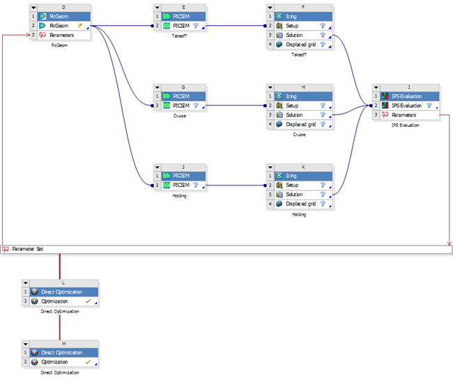
The Workbench user-interface allows you to easily build your project in a workspace called the Project Schematic. To create a general optimization workflow for the piccolo tubes, follow these steps:
If you opened the external-airflow.wbpj project provided with this tutorial, go to step 2. You will use the airflow and water droplet solutions computed in the systems of this project. Otherwise, conduct the simulations described in Setting up the External Airflow and Droplet Impingement Systems.
For each Fluid Flow – Icing (FENSAP) system, specify the external grid (oneram6.grd) of this simulation. This grid is in the Grid folder of your working directory. To select this file, right-click the Setup Flow cell and select Define from file… and go to the location mentioned previously. Copy the grid in each system directory.
Save the project as
ONERAM6-IPSOPTin a preferred user path location.From the Toolbox, drag PicGeom located under IPSOPT Components and drop it in the Project Schematic window under the Fluid Flow - Icing components. Optionally, you can double-click PicGeom in the Toolbox.
Since for each icing condition there is an internal bleed-air condition with specific total pressure and total temperature properties, each condition will have a unique internal HTC. Therefore, in this project, add 3 PICSIM components since there are 3 in-flight icing conditions in Table 1.2: Flight and Icing Condition Matrix. To do this, drag PICSIM located under IPSOPT Components and drop it in the Project Schematic window to the right of the PicGeom component. Repeat this step twice such that they are one underneath the other. From top to bottom, name these PICSIM components
Takeoff,CruiseandHolding(see Figure 1.7: Project of Schematic Workflow).Likewise, 3 Icing components should be connected to their corresponding PICSIM component. To do this, drag the Icing component located under FENSAP-ICE Components in the Project Schematic window. Put them to the right of their corresponding PICSIM component. From top to bottom, name these Icing components
Takeoff,CruiseandHolding.Drag the IPS Evaluation component located under IPSOPT Components to the right side of the Icing components.
Connect PicGeom cell D2 to all PICSIM cells (E2, G2, J2) and each PICSIM cell to its associated Icing Setup cell (F2, H2, K2). Connect each Icing Solution cell to the IPS Evaluation cell (I2). See Figure 1.7: Project of Schematic Workflow.
Note:
A transfer data connection is represented in the Project Schematic by a line with a circle on its right (target) side.
To connect one system to another, click a cell in one system, then drag and drop this cell onto a compatible cell in another system.
The following sections of this chapter are:
The PicGeom component provides piccolo tube geometrical/design parameters to PICSIM. Some of the parameters are user-inputs that remain unchanged during the optimization and some of them are defined as design variables which are updated at every optimization loop.
Follow the instructions below to set up PicGeom:
Select the PicGeom cell. The properties window of PicGeom will appear on the right.
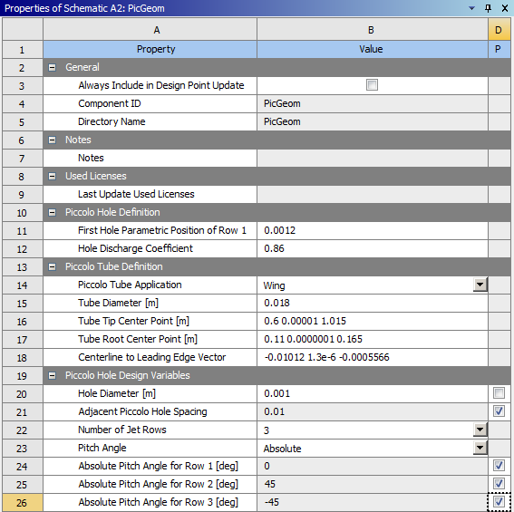
In the Piccolo Hole Definition task group, change the First Hole Parametric Position of Row 1 to
0.0012and retain the default Hole Discharge Coefficient value at0.86.Note: In a three row piccolo hole configuration, row 1 corresponds to the middle row, row 2 represents the upper row and row 3 represents the lower row (see Figure 1.4: Schematic of a Piccolo Tube).
In the Piccolo Tube Definition task group, choose Wing under Piccolo Tube Application and set the piccolo tube geometric parameters using the values shown in the following table:
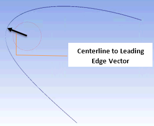
Tube Diameter (m) 0.018Tube Tip Center Point (m) 0.60.000011.015Tube Root Center Point (m) 0.110.00000010.165Centerline to Leading Edge Vector -0.010121.3e-6-0.0005566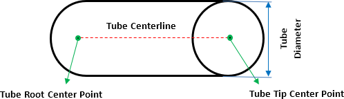
In the Piccolo Hole Design Variables task group, keep the default value of 0.001 m for the Hole Diameter. Select 3 as Number of Jet Rows and Absolute as Pitch Angle type. Keep the default values for Absolute Pitch Angle for Row and Adjacent Piccolo Hole Spacing.
In this tutorial, Adjacent Piccolo Hole Spacing and Absolute Pitch Angle for Row 1, 2 and 3 are design variables. To define them as design variables, select the check box of these parameters. A Parameters cell is automatically created in this component.
Note:
If the geometric parameter of the piccolo tube is a design variable, it will be initialized inside DesignXplorer based on the design variable bounds provided. Therefore, you do not need to specify the initial value for these parameters here.
The Genetic Algorithm optimization method (MOGA) is used as a global search method to find the best optimal solution. This method does not require an initial design to start the optimization process since it is not gradient-based and it creates the design points from the Genetic Algorithm criteria and design space dimensions. Hence, the initial guess or starting point of the optimization process does not correspond to the default value of the design parameters inside PicGeom.
The Adjacent Piccolo Hole Spacing corresponds to the non-dimensional distance between two adjacent piccolo hole centers on the same row. The distance between adjacent holes is non-dimensionalized with respect to the extended length of the tube.
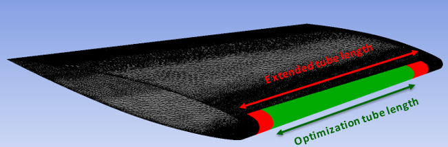
Note: The objective function(s), in this case mass flow rate, and design variables are applied over the entire piccolo tube including the extensions. The constraints are only applied over the protected area without extension.
Takeoff
First, increase the number of significant digits shown in Workbench. Flow properties such as thermal conductivity will require more than the default number of significant digits provided by Workbench. To do this, go to Tools → Options… → Appearance. On the right side of the Options window, scroll down the table and change the Number of Significant Digits under Display to
10. This number is the maximum level of precision of Workbench.Select the PICSIM cell of the first condition (Takeoff). The Properties window of PICSIM will appear on the right.
Link the icing solutions and conditions of the Fluid Flow-Icing (FENSAP) to PICSIM. To do this, click the Fluid Flow-Icing (FENSAP) cell of the Takeoff condition. In the Properties of Schematic window, under the General task group, copy the System ID which, in this case, is ICING_FENSAP.
Copy this System ID, ICING_FENSAP, in Properties of Schematic E2: PICSIM → Wet Air Condition → Source.
Change the Total Temperature and the Total Pressure to
470K and230,000Pa respectively.Change the Thermal Conductivity to
0.036486574W/mK.Change the Kinematic Viscosity to
2.561e-05m2/s.
Cruise
Select the PICSIM cell of the second condition (Cruise). The Properties window of PICSIM will appear on the right.
Click the Fluid Flow-Icing (FENSAP) cell of the Cruise condition. In the Properties of Schematic window, under the General task group, copy the System ID which, in this case, is ICING_FENSAP 1.
Copy this System ID in Properties of Schematic G2: PICSIM → Wet Air Condition → Source.
Change the Total Temperature and the Total Pressure to
450K and170,000Pa respectively.Change the Thermal Conductivity to
0.035353837W/mK.Change the Kinematic Viscosity to
2.4847238E-05m2/s.

Holding
Select the PICSIM cell of the third condition (Holding). The Properties window of PICSIM will appear on the right.
Click the Fluid Flow-Icing (FENSAP) cell of the Holding condition. In the Properties of Schematic window, under the General task group, copy the System ID which, in this case, is ICING_FENSAP 2.
Enter this System ID in Properties of Schematic J2: PICSIM → Wet Air Condition → Source.
Change the Total Temperature and the Total Pressure to
450K and180,000Pa respectively.Change the Thermal Conductivity to
0.035353837W/mK.Change the Kinematic Viscosity to
2.4847238E-05m2/s.
Note:
The CAD and mesh of the protected zone should be separated into 2 groups: the upper surface group and the lower surface group. Each group can contain different wall boundary IDs. The boundary IDs of each group should be defined inside the Grid Task of each PICSIM component under Upper Surface/Inner Barrel Protected Area Boundary IDs and Lower Surface/Outer Barrell Protected Area Boundary IDs.
To optimize the piccolo tube design on a limited portion of the protected zone while considering the effects of a continuous IPS along the span of the wing, it is important to enable the Protected Area Extension and to specify the non-dimensional length of the extended zones to be added on both sides of the protected surface, using the piccolo tube length as the reference length. These end-zones, marked as Extension of Protected Area, will represent the portion of the IPS outside the optimization zone during your calculations.
Data regarding the specific location of each piccolo hole is printed in holes_pos, one of the output files of PICSIM.
Select the Icing Setup cell of the first condition (Takeoff). The Properties window will appear on the right.
Choose Model → Heat flux type → Classical.
Change the Recovery factor to
0.9.Disable the Grid Displacement under the Solver task.
Select the Icing Solution cell and change the number of CPUs to
4.Repeat the same setup (steps 1 and 2) for the remaining Icing components, Cruise and Holding.
Note: The in-flight icing conditions of the Fluid Flow-Icing (FENSAP) have been linked to their respective Icing components via PICSIM.
Select IPS Evaluation cell, I2. The Properties window will appear on the right.
Under the Running Wet Scenarios task group, select the optimization scenario by defining constraint(s) and objective(s). Ice Control is always active during the optimization workflow. It is possible to limit ice formation by specifying a Minimum Skin Temperature, Total Mass of Ice or Maximum Ice Thickness inside the protected area. In this tutorial, Minimum Skin Temperature is selected as a constraint to limit ice accretion over the protected area. To do this, choose Ice Control → Minimum Skin Temperature.
Keep the Minimum Allowable Value (K) as default,
276K. The minimum temperature should be higher than the freezing temperature (273.15 K) to prevent ice formation over the protected area.The IPS Evaluation component supports 4 ways to control the amount of water runback at the end of the protected area. In this tutorial, the ultimate goal of the optimization is to prevent water runback past the protected zone located on the upper surface of the wing, whereas water film that flows past the limit of the protected zone on the lower surface of the wing may be tolerated. To specify these constraints, choose Water Runback Control → Wing Upper Surface/Nacelle Inner Barrel under the Running Wet Scenarios task group.
Enable the Maximum Skin Temperature Control to impose a constraint on the maximum skin temperature to prevent structural weakening. Enter
440K as the Maximum Allowable Value (K).The optimal piccolo tube design should satisfy all constraints while minimizing the bleed-air mass flow rate required to protect the wing. To do this, keep the Objective Function as default: Piccolo Supply Air → Minimum Total Mass Flow Rate.
Check all the boxes that appeared under Objective Functions and Optimization Constraint Functions task group. A Parameters cell is automatically created in this component.
Note: All constraints and objectives that have been selected in the Running Wet Scenarios and Objective Functions are shown under the Optimization Constraint Functions and Objective Functions task groups with boxes besides their names. By checking these boxes, the constraints and objectives become output parameters that can later be used in DesignXplorer.
Workbench uses parameters and design points to either run optimizations or parametric studies to further investigate the performance of the IPS. Once you have defined parameters for your system, a Parameters cell is added to the system/component and the Parameter Set bus bar is added to your project. Arrows representing input and output parameters connect the bus bar to each system in which parameters have been defined.
You can double check the parameter definitions by double-clicking the Parameter Set bus bar. The Parameters Set tab includes the Outline of All Parameters table that lists all the parameters in your project as well as the Table of Design Points in which you can specify design points.
In this case, PICGEOM Parameters are Input Parameters (Design Variables) and the IPS Evaluation Parameters are Output Parameters (Constraints & Objectives) to the optimization workflow.
After setting up all systems and parameters, the design exploration system must be added to the workflow to define the optimization method, the design variable bounds and the type of constraints and objectives that will be used.
To optimize the design of piccolo tube system, you should use the Goal-driven direct optimization method. To take advantage of both global and local optimization methods while minimizing their disadvantages, a hybrid optimization method that combines the Multi-Objective Genetic Algorithm (MOGA) and the Gradient Descent Method (MISQP) is used.
In this manner, the global search method (GA) finds the global optimum and, after convergence, the best candidate point is provided to the local search method (MISQP) to search for the local optimum.
Drag the Direct Optimization component located under Design Exploration and drop it below the Parameter Set bus bar in the Project Schematic. Optionally, you can double-click the template in the Toolbox.
Double-click the Optimization cell of the Direct Optimization component to open its component tab, L2: Optimization. Optionally, you can right-click the Optimization cell and select Edit.
This component tab has four views/windows: Outline, Table, Properties and either Chart or Results. Go to the Outline window and select Optimization to configure the optimization analysis. Selecting items within the Outline window will automatically update the other windows giving you access to the settings of these items.
Activate the advanced options of DesignXplorer. To do this, choose Tools → Options… → Design Exploration and activate Show Advanced Options. The advanced options are shown in Italic format in the Properties window and are needed in this tutorial.
In the Properties window, under Optimization:
Go to Method Selection and choose Manual.
Select MOGA as optimization Method Name. The MOGA method is a Multi-Objective Genetic Algorithm which supports multiple objectives and constraints and aims at finding the global optimum.
Change the Type of Initial Sampling to Optimal Space-Filling.
Change the Number of Initial Samples to
200and the Number of Samples Per Iteration to100.Enter
99for the Maximum Allowable Pareto Percentage and0.0001for the Convergence Stability Percentage. These two parameters control the convergence of the optimization method. Large Pareto percentages and small convergence stability percentages will prevent premature termination of the optimization process.Change the Maximum Number of Iterations to
13. You can still interrupt the optimization before completion if the convergence level is considered acceptable.Increase the Mutation Probability to
0.05.Enter
1under Maximum Number of Candidates, since the current optimization scenario has only one objective. This parameter does not affect the optimization and the generation of the response surface, so it can be changed at the end of the optimization to update the post processing.Note: The recommended number of candidate points depends on the selected optimization method. In general, only one candidate is needed for gradient-based or single objective methods. For multiple-objective methods, there are several potential candidates for each Pareto Front; therefore, the Maximum Number of Candidates should be greater than one.
In the Outline window, select Objectives and Constraints under Optimization to define the design goals and constraints.
In the Table window:
Go to cell B3 and select min_mass_flow as Parameter. Choose Minimize as the Objective Type.
Go to next row and select const_min_temp as Parameter. Choose Values <= Upper Bound as the Constraint Type with an Upper Bound of
0.Go to the next row and select const_max_temp as Parameter. Choose Values <= Upper Bound as the Constraint Type with an Upper Bound of
0.Go to the next row and select const_ushf_only as Parameter. Choose Values <= Upper Bound as the Constraint Type with an Upper Bound of
0.
Note: The Type of the constraint in DesignXplorer, regardless of what constraint you choose, should always be Values <= Upper Bound = 0. You should use this type of constraint since it improves the stability of the optimization methods during convergence. Follow this recommendation, even if the physical constraints cannot be lower than zero.
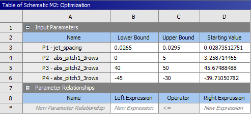
In the Outline view, under the PicGeom node, 4 design variables are listed and correspond to the variables that were checked inside the PicGeom component located in the Project Schematic window. Specify a different set of lower and upper bounds for each of these variables to constraint the design space. To do this:
Select jet_spacing and, in the Properties view, change the Lower Bound to
0.01and Upper Bound to0.03.Select abs_pitch1_3rows and, in the Properties view, change the Lower Bound to
-10deg and Upper Bound to10deg.Select abs_pitch2_3rows and, in the Properties view, change the Lower Bound to
25deg and Upper Bound to50deg.Select abs_pitch3_3rows and, in the Properties view, change the Lower Bound to
-70deg and Upper Bound to-25deg.
When you complete the setup, save the Workbench project.
Go to the Project Schematic window and click the Update Project icon located above this window to run the optimization case.
Note: By default, Workbench only saves the calculated data of the first or current design point, if you want to save the data of all calculated design points within the project to post process the results, go to the Outline view, select Optimization and enable Preserve Design Points After DX Run and Retain Data for Each Preserved Design Point located in the Properties view under Design Points.
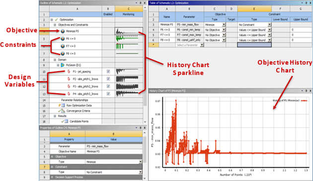
The history chart allows you to monitor the evolution of enabled objective(s), constraint(s) or input parameter(s) through an optimization evaluation and to monitor the convergence of the functions. You can select a different object at any time during the optimization to plot and view the history chart. In the Outline view, a sparkline version of the history chart is displayed for each objective, constraint or input parameter. The history charts will be available even after the update is completed and optimization process is finished.
To access the history chart, select an objective or constraint under the Objectives and Constraints node in the Outline view for the Optimization cell. Alternatively, you can select the design variables under the Domain node.
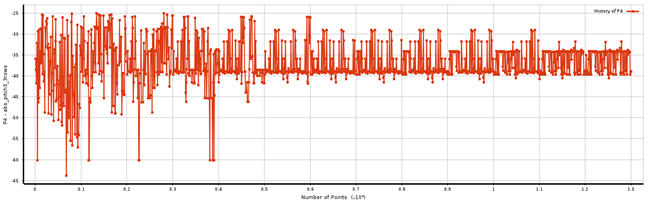
The History charts of our optimization scenario is shown in the following figure. The History chart sparkline is identical to the History chart in the Chart view. Sparklines are green when the constraint is met (values equal or below zero) and are red if the constraint is not met (greater than zero). Gray dashed lines represent bounds for constraints dividing the feasible and infeasible domain.
The number of design points that have been evaluated successfully are shown along the X axis and the objective value is shown along the Y axis. The red line shows the evolution of the objective value. By placing the mouse cursor on any data point on the chart, you can view the X and Y coordinate values.
In the Outline or Chart view, the history chart of the objective Minimize P5 shows that the objective has converged to the best feasible design point.
In the Outline view, the sparklines of the constraints P6 <=0 and P7 <=0 are both red and green, indicating that the constraints were violated at some points and met at others. However, at convergence, the best feasible solution satisfies these constraints.
In the Outline view, the sparkline of the constraint P8 <=0 is entirely green with zero value, indicating that the constraint is satisfied at all design points.
The following charts illustrate the convergence history of the objective, constraints and design variables.
Figure 1.8: Convergence History of the Objective, Minimization of the Piccolo Tube Mass Flow Rate, MOGA Optimization
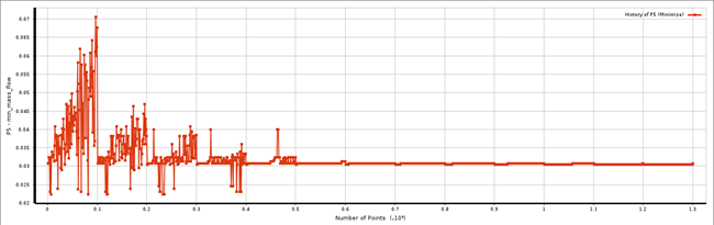
Figure 1.9: Convergence History of the Minimum Relative Wall Temperature Constraint, MOGA Optimization
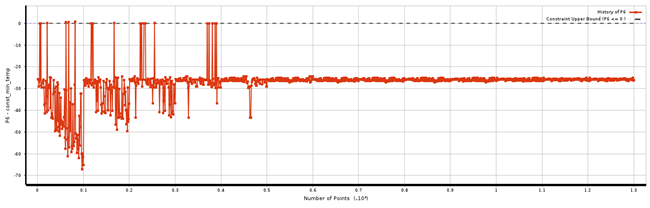
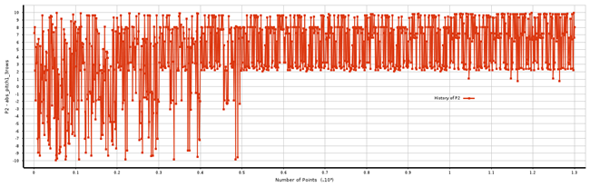
Figure 1.10: Convergence History of the Maximum Relative Wall Temperature Constraint, MOGA Optimization
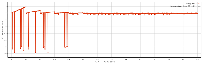
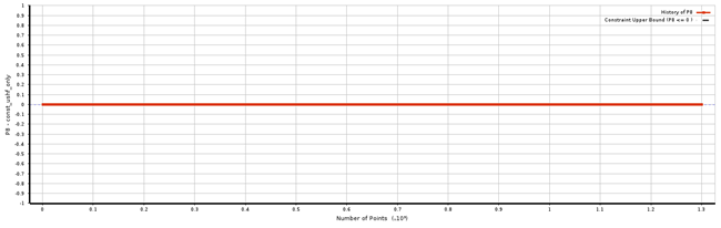
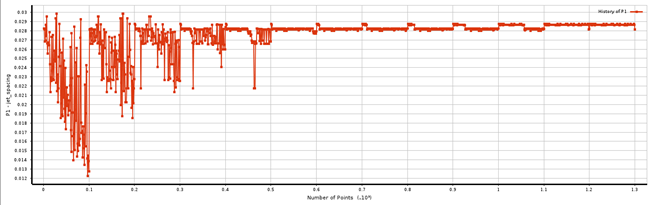
Figure 1.12: Convergence History of the Center-To-Center Jet Spacing Design Variable, MOGA Optimization
Note:
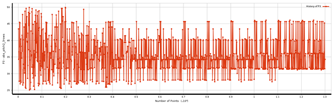
In this specific scenario, the pitch angles vary as the simulation converges towards the optimal mass flow rate, while all constraints and jet spacing converge towards specific values. This behavior reveals that there is more than one pitch angle configuration that satisfies the optimization scenario. If you change the number of candidate points from 1 to 5, you will see different pitch angle configurations with almost the same jet spacing and mass flow rate that satisfy all constraints. Secondly, this indicates that three rows of piccolo holes are more than enough to satisfy all constraints while minimizing the available mass flow rate. Therefore, it is likely that two rows or even one row of piccolo holes will be more appropriate for this optimization scenario. The solution of the optimal two-row configuration is shown in Appendix A.
When carrying out single-objective optimizations, if large oscillations in jet spacing and/or hole diameter are observed in the last iterations or genetic algorithm population, add more MOGA iterations to converge towards the best candidate point. This is usually an indication that the minimum mass flow rate did not properly converge, because the mass flow rate is influenced by these two parameters.
To monitor the design points dynamically as the data are submitted for update, select Raw Optimization Data under the Optimization cell in the Outline view. The Table view will display the raw data of the design points that have been evaluated along with their associated values of constraints, objective and design variables.
It is possible that during the optimization, some of the design points, which are not physically or analytically feasible, fail. In such instances, these points will have a red cross sign in their output parameters and error messages will appear in the message box.
In the MOGA-based multi-objective method, the convergence criteria are defined by the Maximum Allowable Pareto Percentage and the Convergence Stability Percentage. The Maximum Allowable Pareto Percentage criterion looks for a percentage that represents a specified ratio of Pareto points per Number of Samples Per Iteration. When this percentage value is reached, the optimization simulation has converged. The Convergence Stability Percentage criterion looks for population stability, based on mean and standard deviations of the output parameters. When a population is stable with regards to its previous population, the optimization simulation has converged. For detailed information regarding the convergence criteria, consult the DesignXplorer User's Guide .
The output the chart, as shown below, can be displayed in the Convergence view by selecting the Optimization cell located under the Outline view.
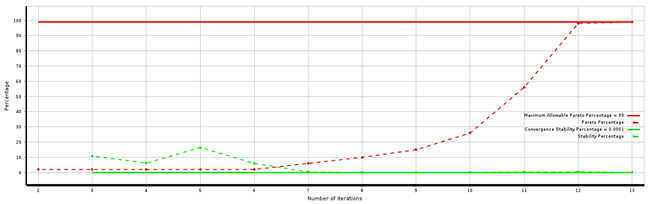
In this chart, the Number of iterations is shown along the X axis and convergence criteria percentage is displayed along the Y axis. The solid red line represents the Maximum Allowable Pareto Percentage which in this case is 99% and the dashed red line represents the evolution of the Pareto percentage. The solid green line is the Convergence Stability Percentage which is 0.0001% in this case and the dashed green line is the stability percentage.
This case converged after 1291 evaluations. You can find this information in Table view. The Table view contains also information regarding the candidate point(s). Scroll down this view to examine the best candidate point of this tutorial. The constraints are all lower or equal to zero. This indicates that the design candidate point satisfied all constraints.
Note:The constraint on minimum temperature is computed using the following equation
where the
 corresponds to the Minimum Allowable Value (K)
which is defined in IPS Evaluation (in this case, its value was set
to 276 K) and
corresponds to the Minimum Allowable Value (K)
which is defined in IPS Evaluation (in this case, its value was set
to 276 K) and  corresponds to the minimum skin temperature of the best candidate
point (276K - (~-25.6771K) = ~301.6771 K).
corresponds to the minimum skin temperature of the best candidate
point (276K - (~-25.6771K) = ~301.6771 K).The constraint on maximum temperature is computed using the following equation,
where the
 corresponds to the Maximum Allowable Value (K)
which is defined in IPS Evaluation (in this case, its value was set
to 440 K) and
corresponds to the Maximum Allowable Value (K)
which is defined in IPS Evaluation (in this case, its value was set
to 440 K) and  corresponds to the maximum skin temperature of the best candidate
point (440K + (~-0.5453 K ) = ~439.4547 K).
corresponds to the maximum skin temperature of the best candidate
point (440K + (~-0.5453 K ) = ~439.4547 K).
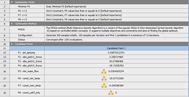


Figure 1.16: Candidate Points Table shows that the optimized piccolo tube mass flow rate (≈0.03 Kg/s) is reduced by approximately a factor of two compared to the highest mass flow rate (≈0.07 Kg/s) computed during the design optimization.
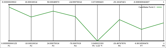
To activate the Candidate Points Chart View, select Candidate Points under Results in the Optimization cell of the Outline view. When the optimization simulation is complete, and results are generated, you can adjust the data presented in this Chart by modifying its settings located in its corresponding Properties view.
The Tradeoff chart is a scatter chart representing the generated design points in the last population. You can find it under Results in the Optimization cell: Optimization → Results → Tradeoff. Point colors in the Chart view show the design points of the last population. The best design points are colored in blue while the worst design points are colored in red. You can display this chart in 2D or 3D by selecting 3D in Mode located under Chart of the Properties view. The 3D chart displays the tradeoff between 3 parameters. Select which parameter to display in the 3D chart by changing one of its axis value located in the Axes cell of the Properties view.
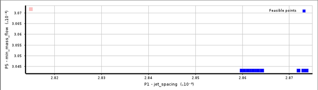
Note: Only feasible points are shown in the Tradeoff Charts.
The following chart shows the relation between jet spacing and the mass flow rate. This chart shows that there are multiple jet spacings that satisfy the minimum mass flow rate. It is important to point out that the variation in jet spacings is small enough that it does not affect the total number of piccolo holes, therefore the mass flow rate.
After completing the MOGA optimization, follow these steps to set up the local optimization method MISQP.
Drag the Direct Optimization component under Design Exploration and drop it below the MOGA Direct Optimization component in the Project Schematic.
Double-click the Optimization cell of the Direct Optimization component to open its component tab. Optionally, you can right-click the Optimization cell and select Edit.
This component tab has four views/windows: Outline, Table, Properties and either Chart or Results. Go to the Outline window and select Optimization to configure the optimization analysis. Selecting items within the Outline window will automatically update the other windows, giving you access to the settings of these items.
In the Properties view, under Optimization:
Go to Method Selection and choose Manual.
Select MISQP as the optimization Method Name. MISQP stands for Mixed-Integer Sequential Quadratic Programming and is a gradient-based method. It only supports single objective optimization problems with multiple constraints. The starting point must be provided to determine the region of the design space to explore. In this case, the starting point corresponds to the best global point given by the Genetic Algorithm method MOGA.
Change the Finite Difference Approximation to Central.
Change the Initial Finite Difference Delta (%) to
10.Modify the Allowable Convergence (%) to
1e-06.Change the Maximum Number of Candidates to
1.
In the Outline view, select Objectives and Constraints under Optimization. The design goals can then be defined in the Table view.
In the Table view:
Select min_mass_flow as Parameter. Choose Minimize as the Objective Type.
Go to the next row and select const_min_temp as Parameter. Choose Values <= Upper Bound as Constraint Type with an Upper Bound of
0.Go to the next row and select const_max_temp as Parameter. Choose Values <= Upper Bound as Constraint Type with an Upper Bound of
0.Go to the next row and select const_ushf_only as Parameter. Choose Values <= Upper Bound as Constraint Type with an Upper Bound of
0.
In the Outline view, under the PicGeom node:
Select jet_spacing and, in the Properties view, change the Upper Bound to
0.0295and the Lower Bound to0.0265. Copy the jet_spacing value from the MOGA candidate point and paste it in Starting Value of the Properties view.Select abs_pitch1_3rows and, in the Properties view, change the Upper Bound to
5deg and the Lower Bound to0deg. Copy the abs_pitch1_3rows value from the MOGA candidate point and paste it in the Starting Value of the Properties view.Select abs_pitch2_3rows and, in the Properties view, change the Upper Bound to
50deg and the Lower Bound to40deg. Copy the abs_pitch2_3rows value from the MOGA candidate point and paste it in the Starting Value of the Properties view.Select abs_pitch3_3rows and, in the Properties view, change the Upper Bound to
-30deg and the Lower Bound to-45deg. Copy the abs_pitch3_3rows value from the MOGA candidate point and paste it in the Starting Value of the Properties view.The figure below shows these settings in the Table view. In this case, the bounds of the design parameters have been narrowed down around the MOGA candidate point to refine the search of the best candidate.
When you complete the setup, save the Workbench project.
Go to the Project Schematic window and click the Update Project icon located above this window to run the optimization case.
Note: By default, Workbench only saves the calculated data of the first or current design point, if you want to save the data of all calculated design points within the project to post process the results, go to the Outline view, select Optimization and enable Preserve Design Points After DX Run and Retain Data for Each Preserved Design Point located in the Properties view under Design Points.
Access the history chart of an objective, constraint or design parameter by clicking its name in the Outline view. At convergence, the following history charts are generated.
These History charts reveal that the MISQP approach found a candidate point with lower mass flow rate than the MOGA method by slightly changing the pitch angles and the spacing of the piccolo holes while respecting all constraints.
Figure 1.17: Convergence History of the Objective Function, Minimize Piccolo Tube Mass Flow Rate in MISQP Optimization
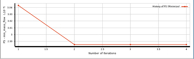
Figure 1.18: Convergence History of the Center-To-Center Jet Spacing Design Variable in MISQP Optimization
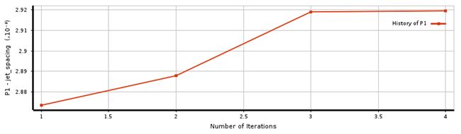
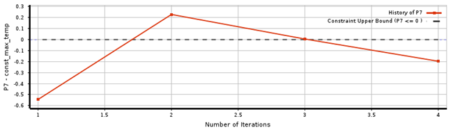
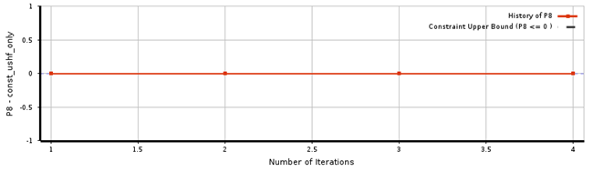
Figure 1.21: Convergence History of the Pitch Angle of Jet Row 1 Design Variable in MISQP Optimization
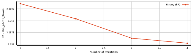
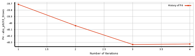
Figure 1.22: Convergence History of the Pitch Angle of Jet Row 2 Design Variable in MISQP Optimization
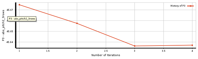
Figure 1.23: Convergence History of the Pitch Angle of Jet Row 3 Design Variable in MISQP Optimization
To monitor the convergence of the objective function, in the Outline view, choose Optimization → Domain → Convergence Criteria.
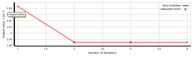
The convergence chart plots the evolution of the best candidate point by identifying the best design point at each iteration.
In this chart, Number of iterations are shown along the X axis and the Output Value (minimum mass flow) is displayed along the Y axis. Red points represent the candidates of each population and gray squares represent infeasible candidates.
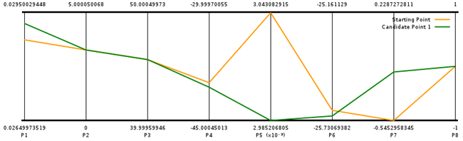
Activate the Candidate Points Chart view by selecting Candidate Points under Results in the Optimization cell of the Outline view. In this case, two curves are plotted; the Starting Point in orange and the Candidate Point in green (see figure below). Starting Point and Candidate Point numerical values can be found in the Table view to precisely evaluate the difference between these two design points.
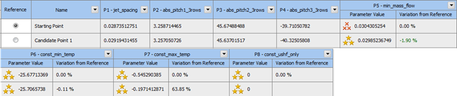
In this manner, the candidate point of the MISQP method represents the most optimal piccolo tube configuration that minimizes the mass flow rate of the bleed-air system and respects all constraints of the condition matrix while keeping the piccolo hole diameter and the piccolo tube position fixed.
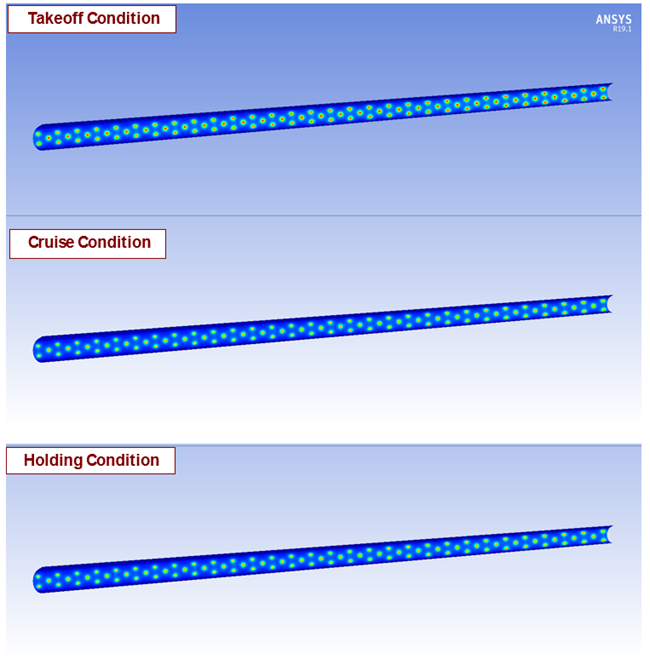
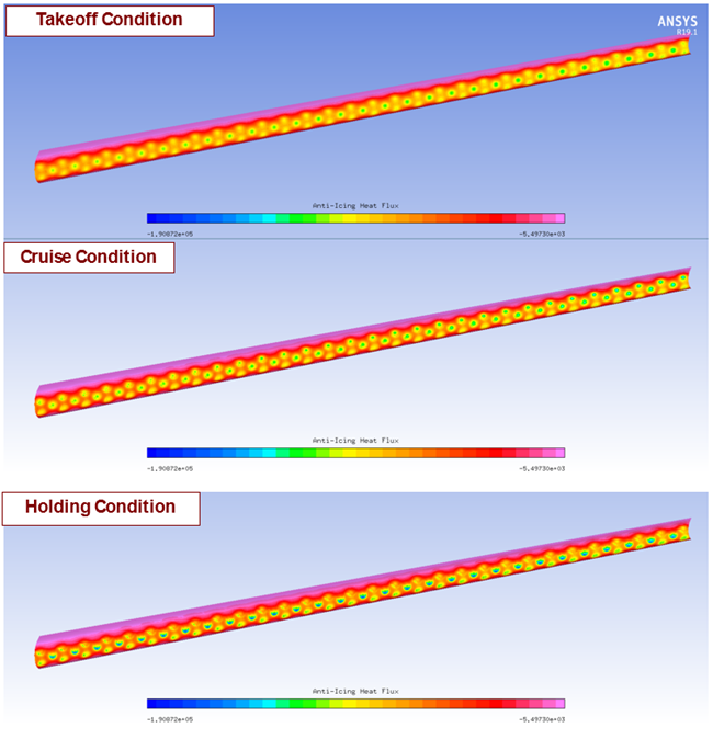
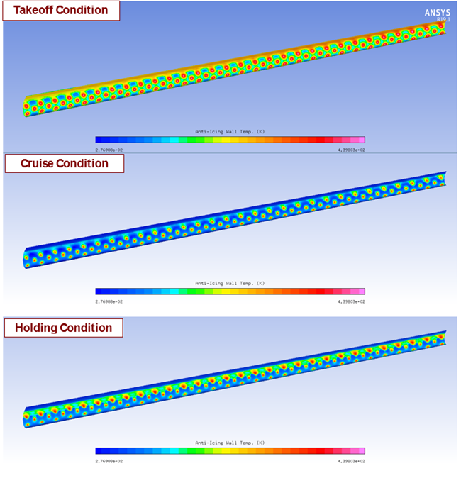
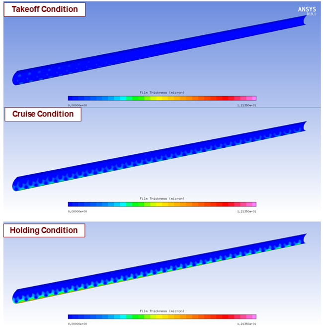
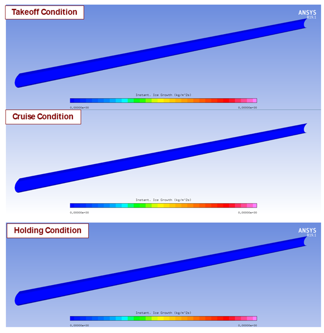
The following figures show the PICSIM and Icing component solutions of the best candidate point produced by the MISQP method. These figures present distributions of Anti-icing HTC (heat transfer coefficients computed by PICSIM), Anti-icing Heat Flux (heat flux provided by the piccolo tube), Anti-Icing Wall Temperature, Film Height and Ice Accretion Rate over the protected zone for all conditions (Takeoff, Cruise, Holding). These figures clearly demonstrate that the constraints of the design case (no ice accretion over the protected zone, no water runback past the upper surface limit of the protected area and wall temperature within 276 K and 440 K) have been met over the protected zone and for all conditions that have been considered in this study.
Note:
At the end of the simulation, the IPSOPT and Icing components do not retain the solutions of the best candidate point. To generate these solutions, a portion of the optimization loop must be created (PicGeom, PICSIM and Icing components) and the design variables of PicGeom should be fixed and set to the design parameters of the best candidate point. Once this is done, update the new system.
To view the Anti-icing HTC, right-click the PICSIM cell and select View solution. The other fields are inside the Icing component solution. Similarly, to the Anti-icing HTC, right-click the Solution cell of the Icing component and select View Solution.