In this verification case, two frictionless spheres with the same radius,
 , are stacked between two fixed walls, causing them to be compressed. The
walls are positioned at
, are stacked between two fixed walls, causing them to be compressed. The
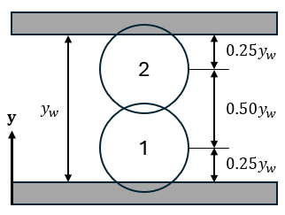
walls are positioned at  m and
m and  , with the particles centers initially located at
  m and
m and  m. This setup, illustrated in Figure 2.23: Compressed spheres stacked between two fixed walls,
ensures the particles remain in contact and under compression.
m. This setup, illustrated in Figure 2.23: Compressed spheres stacked between two fixed walls,
ensures the particles remain in contact and under compression.
A general expression for the acceleration of particle 1 is as follows:
 | (2–21) |
where  is the gravity force,
  is the particle 1-wall spring force,
  is the particle 1-wall damping force,
  is the particle 1-particle 2 spring force and
  is the particle 1-particle 2 damping force.
The expressions for each of these forces are:
 | (2–22) |
 | (2–23) |
 | (2–24) |
 | (2–25) |
 | (2–26) |
where  refers to particle mass,
  is the gravity acceleration,
  refers to spring coefficients, and
  to the damping coefficients.
The  is calculated by:
 | (2–27) |
And the individual  is computed as:
 | (2–28) |
where  refers to Young's Modulus and
  is the particle diameter.
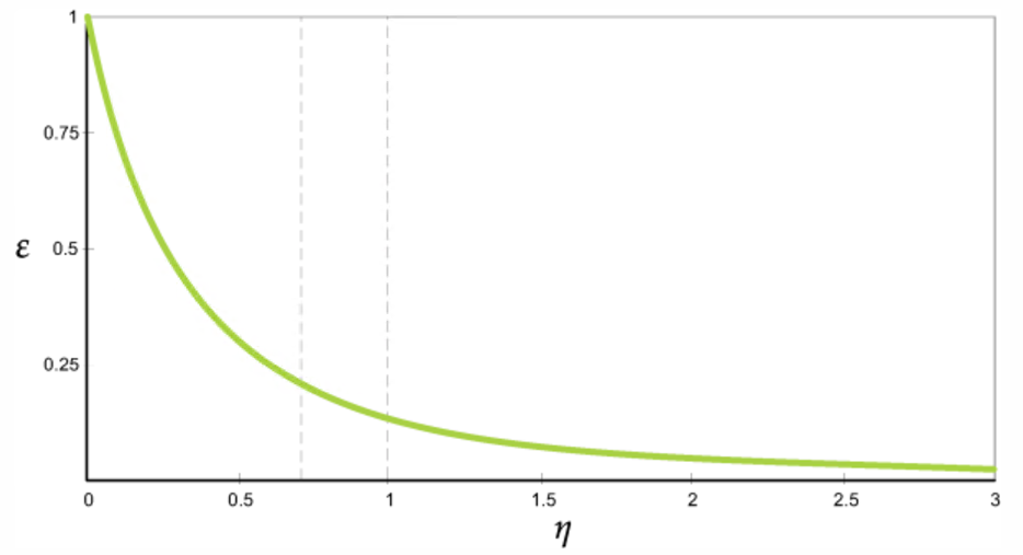
The damping coefficient  is determined directly by the relation shown in the figure below. Refer to
Rocky DEM Technical Manual to see this relation formulation.
is determined directly by the relation shown in the figure below. Refer to
Rocky DEM Technical Manual to see this relation formulation.


The acceleration for particle 1 can be written as:
 | (2–29) |
Similarly, for particle 2:
 | (2–30) |
where the expressions for each of the forces are:
 | (2–31) |
 | (2–32) |
 | (2–33) |
 | (2–34) |
 | (2–35) |
The acceleration for particle 2 can be written as:
 | (2–36) |
This system of equations (Equation 2–29 and Equation 2–36) does not have any known analytical solution so far. However, to be compared with Rocky, it can be numerically solved using the fourth-order Runge-Kutta method.
The equations shown in the last section can be resolved and equivalent results can be calculated by Rocky considering the same input data and boundary conditions. The input parameters for this verification case setup are presented in Table 2.10: Input parameters for the compressed spheres case validation..
Table 2.10: Input parameters for the compressed spheres case validation.
|
Parameter |
Value |
Unit |
|---|---|---|
|
Physical Model: | ||
| Thermal | Disabled | - |
| Normal Force | Linear Spring Dashpot | - |
| Adhesive Force | None | - |
| Restitution Coefficient | 1 | - |
| Gravity Y | -9.81 |  |
|
Particle 1: | ||
| Sphere Radius | 0.0005 |  |
| Sphere Density | 20000 |  |
| Friction Coefficient | 0 | - |
| Young Modulus | 2E06 | Pa |
|
Particle 2: | ||
| Sphere Radius | 0.0005 | |
| Sphere Density | 10000 | |
| Friction Coefficient | 0 | - |
| Young Modulus | 2E06 | Pa |
|
Bottom Wall: | ||
| Friction Coefficient | 0 | - |
| Young Modulus | 2E06 | Pa |
|
Top Wall: | ||
| Friction Coefficient | 0 | - |
| Young Modulus | 2E06 | Pa |
|
Solver Parameters: | ||
| Simulation Duration | 0.001 |  |
| Time Interval | 1E-05 | |
After running the simulations using the parameters described in the previous section, it is possible to compare the results between Rocky and the Runge-Kutta solution. The evolution of the particles positions (measured from their centers) is shown in Figure 2.25: Evolution of the position of particle 1 over simulation time. and Figure 2.26: Evolution of the position of particle 2 over simulation time..
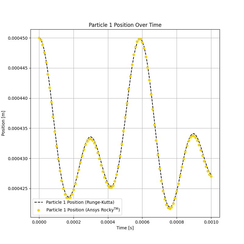
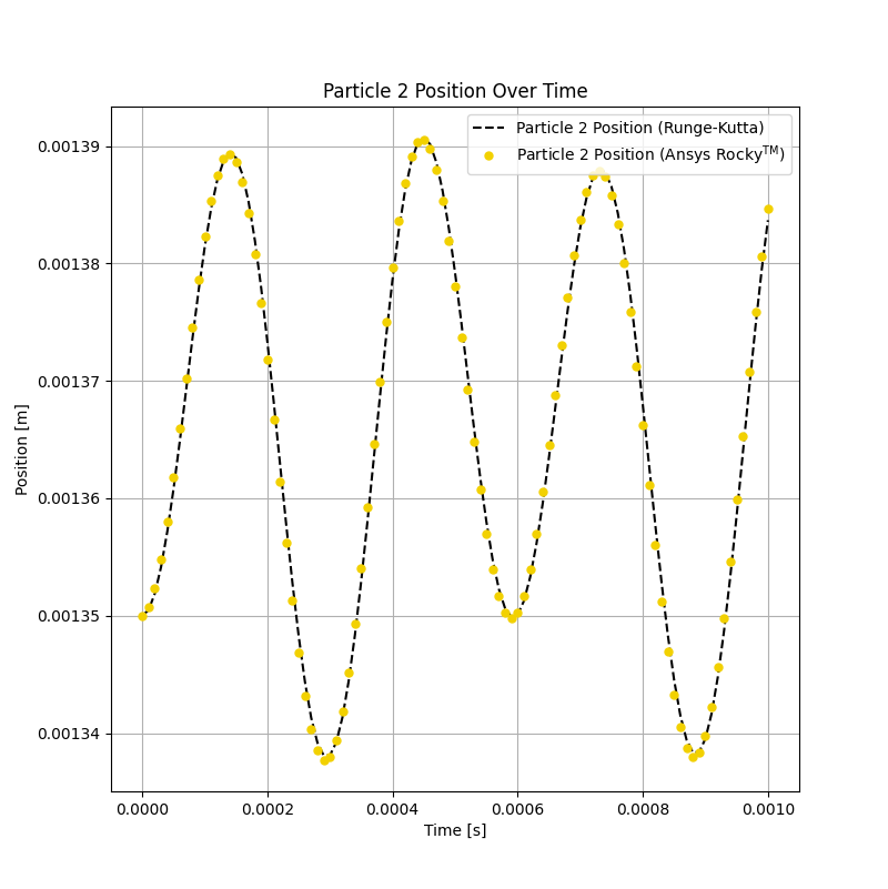
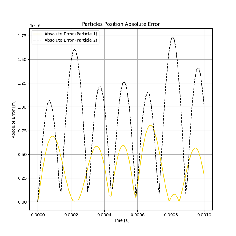
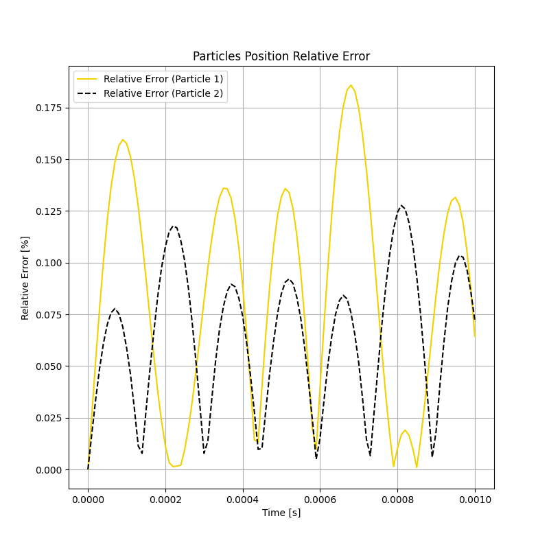
The absolute and relative errors for the particles positions are compared in Figure 2.27: Absolute error between Rocky and Runge-Kutta solution for the particles position. and Figure 2.28: Relative error between Rocky and Analytical solution for the particles position., respectively. The absolute error is maximum for particle 1 around 8.0E-07 m, representing a 0.18% relative error, while for particle 2 it is roughly 1.8E-06 m, representing a 0.13% relative error.