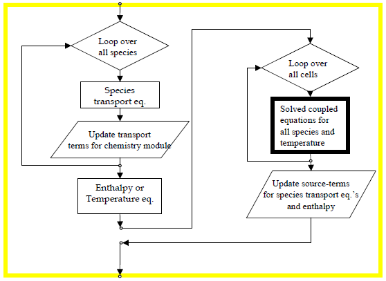
For steady-state problems, the KINetics module includes the option to use a unique approach to the solution of the species conservation equations. This approach provides an efficient way to determine species concentrations in steady state without the need for transient time stepping. The approach is based on an algorithm that alternately solves for all species in each cell, and then solves the same equations, species by species for the entire domain. The flow chart in Figure 2.2: Steady-state algorithm implemented using Chemkin-CFD for determining species concentrations in multi-component systems with CFD simulations; the bold box represents the KINetics module operations illustrates the algorithm. The KINetics module takes care of the cell-by-cell calculations, as indicated by the bold outlined box in Figure 2.2: Steady-state algorithm implemented using Chemkin-CFD for determining species concentrations in multi-component systems with CFD simulations; the bold box represents the KINetics module operations, for the steady-state option. The module allows the transport software to set the appropriate transport terms needed for robust solution of the steady-state problem in each cell and returns the corresponding source terms for the full species conservation equation. In the KINetics iteration, the transport terms that depend on the species concentration of the cell are included in the equation and in the calculation of the numerical Jacobian that is needed for solution of the matrix equations. This greatly enhances the convergence to a steady-state solution.

As in the operator-splitting method, we split the solution of the species equations into two sequential steps. The first step is done on a cell-by-cell basis by the KINetics module, such that all species equations are solved simultaneously within a cell, but each cell is solved one at a time. The second step is done by the CFD program, and may be done on a species-by-species basis, such that each species equation is solved over the entire computational domain at one time. In that sense, we have two steps in the same way as we did for the operator-splitting method. However there are some key differences from the operator splitting transient method. In this algorithm, we include all of the transport and chemistry terms in both steps. In this way both steps are trying to solve the full species equation for all species under steady-state conditions. The difference between the two steps then is the implicitness of the terms in the equation with respect to the numerical solution method.

For a steady-state Chemkin-CFD calculation, the CFD software passes in two additional terms from the transport terms in the overall species conservation equation. These are 1) the sum of all transport terms that would be off the "diagonal" of the Jacobian entry for each species and 2) the sum of all transport term multipliers of the species concentration in that cell. For example, for diffusive transport terms, we take the definition of the diffusion mass flux and observe that there is a strong dependence of the diffusive flux for each species on the species concentration in the cell. We then split the diffusive mass flux term into the product of two terms: one that we keep constant and one that varies in the chemistry simulation. To illustrate this with an equation, the diffusive flux term may be defined in simplest form (1-dimensional gradient, mixture-averaged diffusion properties) as:

(2–13)

Where is the ordinary diffusion coefficient of species in the mixture and is the species mole fraction, and is the mean molecular weight of the mixture. For the sake of argument, we neglect the gradient in mean molecular weight (second term on the right-hand side). We can then focus in on the mass fraction gradient given in the first term on the left-hand side of Equation 2–13. We start by discretizing the equation, which means replacing the spatial derivative with a discrete value for the change in distance, . This distance could represent, for example, the cell-center to cell-center distance in a one-dimensional computational grid. The result would be:

(2–14)

Next we must specify where on the grid we’re going to evaluate the multipliers that are outside of the parentheses on the right-hand-side of Equation 2–14. Ideally they will be an average of the conditions at and at . For simplicity, however, we will set them to , as follows:

(2–15)

Now if we are solving for the species mass fraction at cell number , then we can write the diffusive flux term as:

(2–16)

where

and

For the Chemkin-CFD calculation, then, the terms and in Equation 2–16 are provided by the CFD program and will be fixed based on the last transport-step iteration, while is allowed to vary during solution for this component. For the CFD transport calculation, the KINetics module returns the chemistry net production rates of all of the species as determined from the chemistry sub-step. These are then fixed for each cell, as the CFD program solves the full species equations throughout the entire computational domain. The diffusive flux terms are allowed to vary as the relative balance between species from cell to cell changes. The convective terms also vary as the species value varies.

For the Chemkin-CFD calculations, the steady-state equations are solved using Ansys’ proprietary steady-state solver TWOPNT ; [5]. TWOPNT is a numerical solution package targeted to 1-dimensional boundary-value problems. The solver uses a modified Newton method to solve a set of differential and algebraic equations in zero or one dimensions. One of the package's unique features is a built-in pseudo time-stepping approach to help condition the initial guess for a steady-state solution. This approach dramatically increases the ability to converge reliably and quickly to a steady-state solution even when the provided bad initial guesses.

The result of using the steady-state algorithm is up to 5 times faster than using a time-stepping approach, even with the use of the operator splitting for the time-stepping method. Compared to other existing models, the new approach would allow solutions to problems where it was previously not possible to get a converged steady-state solution.

Figure 2.1: Typical method for solving mass, momentum, energy, and species equations in commercial computational fluid dynamics

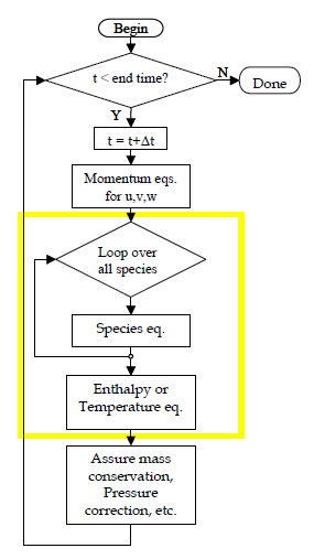
Figure 2.2: Steady-state algorithm implemented using Chemkin-CFD for determining species concentrations in multi-component systems with CFD simulations; the bold box represents the KINetics module operations