


A hydrodynamic analysis allows structures to be connected by articulated joints. These do not permit relative translation of the two structures but allow relative rotational movement in a number of ways that can be defined by the user.
A maximum of 99 joints is allowed.
To add a Joint:
Select the Connections object in the tree view.
Right-click on the Connections object and select Insert Connection > Joint, or click on the Joint icon in the Connections toolbar.
Select the Joint object in the tree and enter the following information:
Type – To add a joint, select the type of joint you are adding:
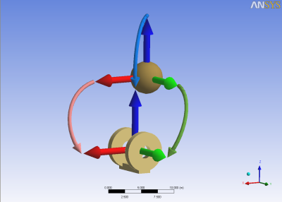
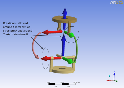
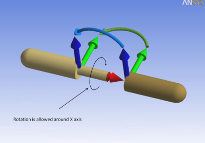
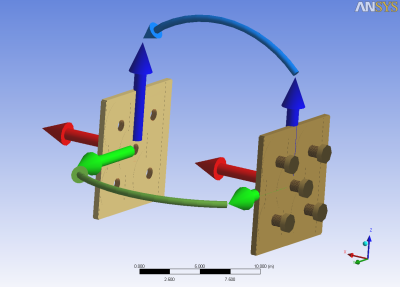
Note: In the following images, the joints are shown with their two ends split apart. Each end is attached to one of the two joint structures (or a structure and a fixed connection point). Each end of the joint has a set of axes attached to it that corresponds to its position with respect to the structure that it is attached to. The curved, colored arrows in the figures below indicate how the two ends will be connected. When the two sets of axes are coincident, the starting position of the structures in the simulation may be different from that in the imported geometry.
Ball and Socket. Free to rotate about all axes.
Universal. Free to rotate about two axes transmitting a moment about the third axis at right angles to the first two.
Hinged. Transmitting a moment about two axes and free to rotate about the third axis at right angles the first two.
Rigid. Transmitting a moment about all three axes and not free to rotate at all. This type of constraint enables you to find the reactions between two or more structures. This type of joint rigidly connects the structures together so that the solution of the equations of motion is the same as if one structure was defined.
In order to see the shape of the connections more easily, you can switch to wireframe mode.
Connectivity – Select the type of connectivity for the joint:
Fixed Point and Structure
Structure and Structure
Fixed Point – For Connectivity of Fixed Point and Structure, select the fixed point from a dropdown list of existing fixed points.
Connection Point on Structure (A/B) – Allows you to select the connection point on the contact structure(s) from a dropdown of existing connection points.
Stiffness About X,Y,Z – These three fields define the rotational stiffness about the X, Y, and Z axes.
Damping About X,Y,Z – These three fields define the rotational damping about the X, Y, and Z axes.
Translation Friction Coefficient – Friction coefficient for transverse force (
 ).
).Rotational Coefficient – Friction coefficient for overturning moment (
 ).
).Axial Friction Coefficient – Friction coefficient for axial force (
 ).
).Constant Friction Moment – Constant friction moment (
 ).
).The frictional moment is given by:
where:
 if the relative rotational velocity is less than 0.001 rad/s, 1
otherwise
if the relative rotational velocity is less than 0.001 rad/s, 1
otherwise are coefficients. These are not conventional dimensionless friction
coefficients, as used in the equation
are coefficients. These are not conventional dimensionless friction
coefficients, as used in the equation  . These coefficients are factors to be applied to the appropriate forces
to give frictional moments, and they must include effects of the bearing diameter etc.
. These coefficients are factors to be applied to the appropriate forces
to give frictional moments, and they must include effects of the bearing diameter etc.
 through
  must not be negative.
  and
and  have dimensions of length, and the maximum value allowed is
 where
where  is the acceleration due to gravity and
  is the acceleration due to gravity in the [kg, meter, second] unit
system.
is the acceleration due to gravity in the [kg, meter, second] unit
system.  is non-dimensional and has a maximum value of 0.025.

When inserting a joint, two axis objects are inserted as its children (Joint Target Axes and Joint Contact Axes). These axes objects define the orientation of the two objects that are connected by the joint. The orientation can be set using these fields in the Details panel for each axes object:
Alignment Method – Select Global Axes to align the axes with the global axes. You can also set the alignment of the axes using the Vertex Selection or Direction Entry methods.
Origin Vertex, X Direction Vertex, Vertex Defining the XY Plane – For an Alignment Method of Vertex Selection, select the Origin Vertex of the axis, a vertex defining the X direction (X Direction Vertex), and a vertex that would, along with the other two vertices, define the XY Plane (Vertex Defining the XY Plane).
Rotation about Global Z, Rotation about Local Y ,Rotation about Local X – For an Alignment Method of Direction Entry, define the alignment using these three rotation fields.
Note: If your joint is connecting the structure to a fixed connection point, it will be indicated by a black sphere. This black sphere is not to be confused with the sphere of a ball and socket joint.
In hydrodynamic analyses, inserting joints between two structures affects the initial position of these structures when the analysis is run.
The program automatically determines the initial positions based on the defined joints so that you do not have to edit the model’s initial geometry. If two connection points are not coincident, the program moves one of the structures to align the connection points before running the analysis. The geometry movement will not be shown in the viewer.
You can control which structure will remain in a defined position and which structure is free to move by selecting Connection Point on Structure A or Connection Point on Structure B in the details dialog for the joint. Fixed connections are shown in black.
The rules for defining fixed and movable structures are as follows:
If neither of the two is connected to a fixed connection point, the structure with the Connection Point on Structure A option will remain at its original position and the structure with the Connection Point on Structure B option will be moved.
The Connection Point on Structure A or Connection Point on Structure B designations will be overridden in some situations. If one of two structures is connected to a fixed connection point or is part of a group of articulated structures that are already connected to a fixed connection point, then that structure will remain in a defined position and the other structure will be moved. If this second structure is also part of a group of articulated structures that are not connected to any fixed connection point, the full group to which this structure is already connected will also be moved. Note that this action is independent of the Connection Point on Structure A or Connection Point on Structure B designations.
If one or both of the structures are part of groups of articulated structures and none of these structures is connected to a fixed connection point, then rule #1 applies and the structure with the Connection Point on Structure B designation will be moved, along with its group of structures.
If both articulated groups are already connected to fixed connection points, the new joint is then going to close the loop. See rules for Closed Loops below.
Structures are moved in two steps: They are first translated, which causes the joint points to be coincident, and then the structures are rotated so that the two sets of axes attached to the joint object become superimposed. This gives you the freedom to set an initial orientation for the structures at the start of the Time History Analysis. You will not see the structures move in the viewer.
The resulting set of axes defines the local joint axes at the start of the Time History Analysis. In this set of axes, some rotational motion of the structures will be allowed during the Time History Analysis, depending on the type of joint selected:
Ball and Socket Joint: all rotations are allowed.
Universal Joint: rotations are allowed around the X and Y axes of the local axes system.
Hinged Joint: rotations are only allowed around the X axis of the local axes system.
Rigid Joint: no rotation is allowed.
In hydrodynamic analyses, the following conditions and recommendations apply to closed loops in articulated groups of structures:
The joint positions in the closed loop must be geometrically compatible. It is not possible to connect two structures using two joints if the distance between these joints is different on both structures.
In some cases, use a single joint of a different type that performs the same function as two simpler joints. For example, two ball and socket joints can be replaced by a single hinged joint or two hinged joints can be replaced by a rigid joint.
A closed loop must not result in any redundancies that result in locking the degrees of freedom.
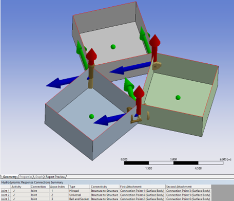
Figure 5.9: A Closed Loop with No Redundant Constraints shows a closed loop joining three wireframe structures. Three articulated structures are connected to form a triangle. One of the joints is a vertical hinged type. The second one is a universal type where neither the joint's local x- nor y-axis is parallel to the line passing through the connection points of the second and third joints. The third one is a ball and socket joint because making it the same as the other joints results in redundancy.
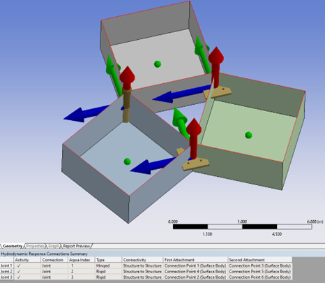
Figure 5.10: A Closed Loop with Redundant Constraints shows a closed loop joining three wireframe structures. The ball and socket and universal joints from Figure 5.9: A Closed Loop with No Redundant Constraints have been replaced by the rigid joints which have added five redundant constraints to the problem. This results in the statically indetermined solution of the reaction forces/moments on the joints.
When you close a loop, a warning message is produced to inform you that a loop is being closed which may cause errors while solving.
Joints can be removed from an analysis temporarily or permanently by right-clicking on the Joint item in the tree and selecting Suppress or Delete. The result is that the group of articulated structures that contains the joint is broken into two parts. Closed loops that are suppressed or deleted are opened.
If the starting positions of some structures were modified when the joint was created, they will be moved again using the following rules:
If the two structures are not part of any group, they will be returned to the positions they held when the geometry was created.
If more than two structures are part of the group to be broken apart, the program positions both subgroup structures where they would have been if the two subgroups had been originally created with the remaining joints. The suppressed and deleted joints are not considered as part of the new arrangement. The existing joints are applied in chronological order.