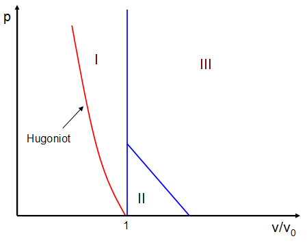
The total range of the pressure-volume plane is divided into four regions as shown in the following figure.

The region to the left of the Hugoniot can only be reached by adiabatic (non-shock) compression and is not relevant to impact problems. It is therefore excluded from the formulation.

Region I represents the compressed phase of the material and extends vertically to shock pressures of about 1000 Mbar.

Region II describes material which has been shocked to an energy less than the sublimation energy e_s and will therefore, on adiabatic release, return to zero pressure as a solid.

There is no provision in this equation of state to describe the material at pressures less than zero.

Region IV is the expansion phase of material which has been shocked to an energy e_s' sufficiently large to ensure that it will expand as a gas at very large expansions.

For convenience the change of phase is assumed to take place at v = v₀.

For large specific volumes, the formulation for Region IV extrapolates to an ideal gas limit.

It is desirable, or even necessary, to ensure that the formulations in each region provide continuous values of the pressure and its first derivatives at the boundaries between contiguous regions.

This is true for the boundary between Regions I and II at v = v₀ but if e_s' is set equal to e_s difficulties may arise at the boundary between Regions II and IV at volumes slightly greater than v₀.

To avoid this problem Region III is defined by setting

(22–1)

where e_v is the vaporization energy at zero pressure determined, like the boiling point energy e_s, from thermodynamic data.

Region III lies between Regions II and IV where e_s < e < e_s'. In this region the pressure is calculated as a mean between that calculated for Regions II and IV.

The constant k is determined empirically to ensure a well behaved solution and in practice satisfactory solutions have been obtained with values of k in the range of zero to one fifth.

In what follows let:

(22–2)

You are prompted for the reference density ρ_ref (or ρ₀ in the equations below) and the constants in the Tillotson equation of state viz. a, b, A, B, α, β, e₀, e_s, and e_s'.

For Region I (μ 0) the pressure p₁ is given by a Mie-Gruneisen equation of state, but since the formulation is to be valid for a very large range of pressure, the Gruneisen Gamma is a function of both v and e, not just a function of v alone.

The constants fit the low pressure shock data but they are adjusted to fit the asymptotic Thomas-Fermi behavior for the variation of pressure at maximum compressions (like a monatomic gas).

The formulation for Region II is as for Region I with a slight modification to one term to avoid difficulties as μ goes increasingly negative.

In Region IV the formulation is chosen to give the correct behavior both at high pressure/normal density and for very large expansion (where it must converge to an ideal gas behavior).

With these constraints the different formulations are:

Region I (μ 0)

The pressure p₁ is given by

(22–3)

Region II (μ < 0, e e_s)

The pressure p₂ is given by the same formulation as that for Region I except that B = 0, i.e.

(22–4)

Region III (μ < 0, e_s < e < e_s')

The pressure p₃ is given by

(22–5)

Region IV (μ < 0, e e_s')

The pressure p₄ is given by

(22–6)

where x = 1 - 1 / η.

The total range of the pressure-volume plane is divided into three regions as shown in the following figure.

The region to the left of the Hugoniot can only be reached by adiabatic (non-shock) compression and is not relevant to impact problems. It is therefore excluded from the formulation.

Region I represents the compressed phase of the material and extends vertically to shock pressures of about 1000 Mbar.

Region II describes material which has been shocked to an energy less than the sublimation energy e_s and will therefore, on adiabatic release, return to zero pressure as a solid.

There is no provision in this equation of state to describe the material at pressures less than zero.

Region III is the expansion phase of material which has been shocked to an energy e_s sufficiently large to ensure that it will expand as a gas at very large expansions.

You are prompted for a Gruneisen Gamma, Γ₀, an expansion coefficient, H (the effective ideal gas constant at large expansions, γ - 1) the sublimation energy, e_s, and constants A₁, A₂, A₃, T₁, and T₂.

Then the formulation is:

Region I (μ 0)

The pressure p₁ is given by

(22–7)

in this equation Γ ρ = Γ₀ ρ₀.

Region II (μ < 0, e < e_s)

The pressure p₂ is given by

(22–8)

If T₁ is input as zero it is reset to T₁ = A₁

Region III (μ < 0, e e_s)

The pressure p₃ is given by

(22–9)

where N = A₁ / ρ₀ Γ e_s.

Unlike the Tillotson EOS, there is no interpolative region between regions II and III.

Key Consideration for Puff EOS

It is important to note that the implementation of the Puff EOS in Autodyn differs from what is described in Bakken & Anderson [4]. The variable ALPHA is used to track the region out of the three described above. Typically, this is an integer (whole) number (see the comment below for Eulerian grids). It effectively determines which equation of state calculation is used as follows:

ALPHA is calculated prior to the calculation of the equation of state and is set to:

If none of the above conditions are met, then the value of ALPHA remains the same as the previous cycle.

An additional note for 3D Eulerian grids is that the value of ALPHA is transported in the advection step of the Eulerian cycle which may result in non-integer values of ALPHA when plotted or examined in the Autodyn GUI.

In the single phase region the behavior of the material is described by a Gruneisen equation of state of the form

(22–10)

where in this case p_r (v), e_r (v) and Γ_r (v) are the tabulated functions along the saturation curve and are determined for a specific value of v by interpolation within the tabular entries.

It is assumed that on the liquid side of the saturation curve T_r, e_r and Γ_r vary quadratically with v_r along the curve and that p_r may be obtained from a relationship of the form

(22–11)

On the vapor side of the saturation curve e_r and Γ_r are taken to vary linearly with T_r, and v_r and T_r are assumed to be related by

(22–12)

and

(22–13)

In the two-phase region below the saturation curve the specific volume v of the liquid-vapor mixture is written as

(22–14)

and the internal energy e as

(22–15)

where α is the mass fraction of vapor in the liquid-vapor mixture and v_g, v_l, e_g and e_l are the specific volumes and internal energies of the saturated liquid and vapor at the saturated vapor pressure p and temperature T, i.e. they are conditions on the saturation curve.

Eliminating α from the two equations above gives

(22–16)

This is an implicit equation defining p (or T) in terms of v and e.

Data on the saturation curve for water has been extracted from Morgan’s paper and included as a standard option in Autodyn.

For any other material you will have to supply the required saturation curve data using subroutine EXTAB (the comments in EXTAB explain how to use this subroutine).

Using the JWL EOS with burn on time provides a good simulation of the detonation process if it is clear that the explosive does indeed fully detonate (release all its chemical energy).

Early experimental work on the initiation of detonation indicated that as a shock front proceeds through a heterogeneous explosive it interacts with local density discontinuities, producing numerous local hot spots that explode but do not propagate.

However energy is released which strengthens the shock so that when it interacts with further non-homogeneities, higher temperatures are produced at these hot spots and more of the explosive is decomposed.

There is thus a run distance for the build-up to detonation and it has been found (Ramsay & Popolato 1965 [6]) that each explosive has a characteristic run to detonation versus shock pressure—the so-called "Pop plots".

Making the further assumption that the explosive passes through the same pressure, distance and state of partial decomposition, regardless of the initial conditions, i.e. that it follows a unique path in distance, time and state space, Forest (Forest 1976 [7]) developed the Forest Fire model to be consistent with the Pop plots by suitable choice of arbitrary coefficients.

This so-called ignition and growth model was not, however, so successful in matching pressure-time data obtained from gauges embedded in the explosive.

A more recent ignition and growth model, the Lee-Tarver model is included in Autodyn.

This model, as with Forest Fire model, is based on the assumption that ignition starts at local hot spots and grows outward from these sites.

The initial version of this model (Lee & Tarver 1980 [8]) described a two-part reaction rate model with a term for ignition of the explosive and a term describing the growth. The reaction rate in this model was given by:

(22–17)

where the compression μ is, as usual,

(22–18)

F was the reaction ratio (ratio of the mass of the gaseous explosive to the total mass of the explosive), p was the pressure in the explosive and I, x, r, G, y, and z were constants. In this model r = 4, so the ignition term depended on the fourth power of the compression of the explosive.

In the more recent model included in Autodyn (Tarver, Hallquist & Erickson 1985 [9]), an additional term is added to overcome the deficiencies of the earlier model in matching data for very short shock pulse initiation.

In this new model, there is a three-fold process of ignition, growth and completion and the reaction rate is given by:

(22–19)

where F, μ and p are defined as above and I, b, a, x, G₁, c, d, y, G₂, e, g and z are constants.

For the explosive PBX-9404, x = 20, so the ignition term depends upon the 20^th power of the compression.

The model described by the above equation gives a very rapid pressure spike on ignition, followed by a slow growth of the reaction that accelerates when the regions around the hot spots coalesce.

In Autodyn, the Lee-Tarver equation of state is used to model both the detonation and expansion of high explosives.

The solid inert explosive is modeled using either a JWL EOS or a shock EOS, while the gaseous expansion products are modeled with the JWL EOS with the reaction rate given by the equation above.

For a more physical post-burn behavior for medium and large expansions, the strength of the material is dependent on the burn fraction, F:

(22–20)

where σ is the current yield strength and σ₀ is the original yield strength of the unburned material.

In the past, the Powder Burn model has also been known in Autodyn as the Slow Burn material model.

Two different formulations of the powder burn model have been implemented, dependent on the material behavior of the reacted (burned) material:

The powder burn model is available for the 2D and 3D structural Lagrange, SPH, and Euler multi-material solver types. For Euler, only the formulation using an Exponential reacted equation of state can be used.

There is a need to numerically simulate the combustion of materials where the dominant physical characteristic of the burning is deflagration rather than detonation of the combustible material. The complicated chemical reactions that dictate the burning of the energetic material are extremely difficult to model from first principles. Therefore, a mathematical model based on the averaged quantities of the governing properties has been proposed [10]. The model was developed using detailed studies of a variety of experiments involving energetic materials where the convective burning front moves behind the pressure front of a shockwave. This type of burning occurs in many incendiary devices and munitions.

Theory

The powder burn model is a multi-phase model where gas and solid can be present in one cell at the same time step. The total mass within each cell is found by added together the mass of the gas and of the solid. The volume taken by the gas and solid are both known and therefore the density, compression, etc., of the material within the cell can be calculated. The burning of the material is dependent on the burn fraction F(t) where,

(22–21)

and

(22–22)

The burning velocity, c(t), is given by a user supplied function, H, dependent on the pressure of the gas,

(22–23)

It has been shown [10] that the burn fraction can be represented as a function of H and a function, G(F(t)), which expresses the size and shape of the burning surface, such that:

(22–24)

The functions G and H are user supplied and are entered in the material data menu, and a typical burn fraction variation in time is shown below:

The burn fraction should only be calculated on the amount of solid material within each cell which has been ignited. Therefore the total burn fraction within each cell, F_t(t) is found by multiplying the burn fraction, F(t), multiplied by the ignition fraction, I(t), such that

(22–25)

The ignition fraction, I(t) is dependent on the velocity of the burn front, V(t), which is also known as ignition velocity and which depends on the equation of state selected by the user for the reacted gaseous material.

When the JWL EOS is selected for the Reacted EOS the ignition velocity is taken constant

(22–26)

and when the Exponential EOS is selected the ignition velocity depends on pressure and density according to:

(22–27)

where C₁, and C₂ are user defined constants, H and γ are user defined functions and ρ_s is the solid density averaged over the cell volume.

The total burn fraction then dictates the amount of solid which is burnt and has changed into a gaseous state at each time step.

When an Exponential reacted EOS is chosen the pressure of the gas, P_g, is calculated as:

(22–28)

where ρ_g is the gas density, e_g the gas internal energy and D is a user defined constant.

The pressure of the solid is evaluated using a separate equation of state, which is user defined and can be either a linear or a compaction EOS. As the solid material burns it changes state such that when the cell is fully burned only gas is present within the cell. A typical density variation in time is shown below,

Material Data Input

Autodyn requires the user to input the values of the burn fraction growth parameters, G and c. These growth parameters are used to evaluate the change in the burn fraction where,

(22–29)

When the JWL EOS is chosen for the reacted gaseous material the constant burn front velocity must be entered as well as the relationship between H and P_g. Because the burn velocity is constant, the ignition time of the elements needs to be defined using the on-time detonation logic.

When the Exponential EOS is chosen for the reacted gaseous materials the constants C₁, C₂, and the relationship between H and P_g must be entered in addition to the variation between density and γ in the relationship below:

(22–30)

Because the burn velocity for this reacted EOS is not constant but varies depending on gas pressure and density, the ignition times for the elements cannot be defined using the on-time detonation logic, and to start the ignition of elements the option of manually setting the detonation (ignition) times needs to be used.

The unreacted solid can be represented using a compaction or linear EOS.

Example

Example application of Powder Burn model used in the Multi-material solver to propel a sabot and projectile inside an experimental gun chamber