


Output
This panel lets you define solution controls for your model.
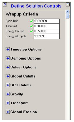
Wrapup Criteria
These controls are the only ones visible when you open this panel for the first time. This is because you must specify some of the parameters (all other control inputs have default values that are usually OK).
Cycle limit
Enter the maximum number of cycles you want your problem to run (enter a large integer if you don't want your problem to stop on a cycle limit).
Time limit
Enter the maximum time you want your problem to run (enter a large number - for example 1.0E20 - if you do not want your problem to stop on a time limit).
Energy fraction
Enter the energy fraction you want to use to stop your problem if the energy error gets too large. The default value of 0.05 causes your problem to stop if the energy error exceeds 5%.
Energy reference cycle
Enter the cycle # at which you want Autodyn to start checking for an energy error.
Press  alongside any of the remaining options to reveal
the input fields for that option :
alongside any of the remaining options to reveal
the input fields for that option :
Timestep Options
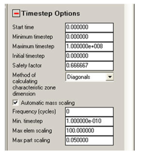
These options control the timestep Autodyn uses to run your problem.
Start time
Enter the start time for your problem.
Minimum timestep
Enter the minimum timestep you want to use.
If the timestep drops below this value, your problem will be terminated.
If you leave this field zero, the minimum timestep will be set to 1/10 of the Initial timestep.
Maximum timestep
Enter the maximum timestep you want to use.
Autodyn will use the minimum of this value or the computed stability timestep.
Initial timestep
Enter the initial timestep you want to use.
If you leave this field zero, the initial timestep will be set to 1/2 the computed stability timestep.
Safety factor
It is not wise to run problem at the stability limit, so a safety factor is applied to the computed stability timestep.
Enter the stability factor you want to use.
The default value (0.6666) is good for all problems, but you may want to increase this value to 0.9 in some cases to use a larger timestep (0.9 is a good value for most Lagrangian calculations).
Method of calculating characteristics zone
Three options are available for calculating the effective zone size used in the timestep calculation. By default, all models will use a zone size calculation based on element diagonals. If you want to obtain improved efficiency, especially in 3D simulations, the zone size calculation can be switched to one of two alternative options (based on either distances between opposing face centers or closest face centers).
To obtain the optimal time step for HEX solid elements the method of calculating the characteristic zone dimension needs to be set to Opposing Faces option instead of the default Diagonal option.
Experience to date has shown that these options can significantly improve the efficiency of Lagrange simulations, especially in 3D. However, in certain circumstances when cells become highly distorted instabilities have been observed causing the calculation to terminate with high energy errors. The correct choice of erosion strain can reduce these problems. It is therefore recommended that users only utilize either of these non-default zone_size options if efficiency is critical.
Automatic Mass Scaling
Mass scaling is an artificial (numerical) mechanism for increasing the CFL (Courant-Friedrichs-Lewy) timestep of individual elements that govern the maximum allowed timestep of explicit transient dynamic solutions in Autodyn. Increasing the timestep has the obvious benefit of reducing the number of cycles required to run a simulation to a given point in time. Educated use of this option can therefore result in significant improvements in efficiency.
Damping Options
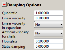
These options control the magnitude of damping applied to your problem.
The default values are best for most problems.
Be very careful if you increase these values, they can significantly change your solution.
Quadratic viscosity
Enter the coefficient of quadratic viscosity you want to apply to shocks (compression waves).
Linear viscosity
Enter the coefficient of linear viscosity you want to apply to shocks (compression waves).
Linear viscosity in expansion
Choose whether you also want to apply the linear viscosity in expansion.
Artificial viscosity for shells
Choose whether to apply artificial viscosity to all structured shells in the model. The linear and quadratic coefficients used are those specified above. You can apply artificial viscosity to an unstructured shell using the Solver Options in the unstructured Parts menu.
Hourglass damping
Enter the coefficient of hourglass damping that you want to apply to Lagrangian elements.
Static damping
A static damping constant may be specified which changes the Autodyn calculation from a dynamic solution to a relaxation iteration converging to a state of stress equilibrium. For optimal convergence, the value chosen for the constant, R, may be defined by:
R=2*timestep/T
where
timestepis the expected average value of the timestep andTis longest period of vibration for the system being analyzed.Note: An Autodyn model that shares a setup with an Explicit Dynamics system that has more than one simulation step will have the static damping coefficient set per step, which is not visible in the Autodyn GUI. In this case, the static damping constant in the Autodyn GUI will display a value of 1e6 to indicate that the static damping coefficient is controlled by the simulation step data. In order to override the per step static damping constants, input the desired static damping constant into the static damping input field in the Autodyn GUI. The constant must be less than 1e6 for it to override the per step data.
Solver Options
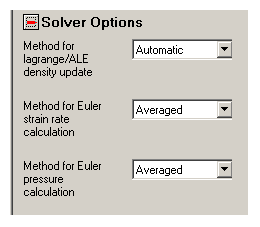
Method for Lagrange/ALE density update
The element density can be updated each cycle using one of two methods; incrementally from the change in volume relative to the last cycle or recalculated based on the current mass and volume of the element. If the incremental change in volume over a cycle is small, it can be more accurate to use the incremental approach rather than the total approach to updating the density.
Hence the options are:
Automatic
Autodyn decides whether it needs to do an incremental update or not based on the change in volume.
Incremental
Force Autodyn to always use the incremental update.
Total
Force Autodyn to always recalculate the density.
Method for Euler Strain rate calculation
For multi-material Euler there are two methods to compute strain rates:
Weighted.
For multi-material Euler analysis, involving materials with strength, strain rates need to be calculated to compute the increment in strain from cycle to cycle. The strain rates are derived from the velocity gradients, which are obtained by an element surface integration of the velocity. Using the Weighted option the face velocity that is used in the integration is a density weighted average of the element velocity on both sides of the face.
This is the default option and provides the most accurate strain rate calculation.
Averaged.
With this option the face velocity used in the integration is a simple average of the element velocity on both sides of the face and provides less accurate results than the Weighted option. Until Autodyn Version 6.1 the Averaged option was the only option available, and can be used to reproduce old results. Also models that are generated before Version 6.1 will still run using the Averaged method.
Method for Euler pressure calculation
For multi-material Euler cells containing two or more materials, there are two methods for calculating the resultant cell pressure:
Equilibrium
An iterative procedure is used for each material in a cell to establish a single pressure consistent with the equation of state and conditions of each material in the cell. This method is currently only applied if there are two materials in the cell and these materials are defined by ideal gas, or fully burnt JWL material. If this criterion is not met in a cell the pressure averaging option is used.
Average
The resultant cell pressure is calculated from a weighted average of the pressure of the individual materials in the cell. The weighting algorithm takes account of both the volume fraction of each material and the relative stiffness of each material. This is the default method.
Global Cutoffs
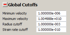
These options let you set global cutoffs.
The default values are usually good if you are using the default units (mm, mg, ms). You may want to change one or more of these defaults if you are using some other set of units.
Minimum velocity
Enter the minimum velocity cutoff you want to use.
If any velocity drops below this value it is set to zero.
Maximum velocity
Enter the maximum velocity you want to use.
If any velocity rises above this value it is set to this value.
This option is sometimes useful if your problem develops high velocities, which result in a small timestep, in regions that are not important to your solution.
Radius cutoff
Enter a value for the radius cut off for 2D axial models.
If a Lagrangian node is inside this radius at the start of your calculation, it is placed on the axis of symmetry.
If a Lagrangian node is outside this radius at the start of your calculation, it will not be allowed to come closer than this radius to the axis of symmetry as your calculation proceeds.
Strain rate cutoff
Enter a value for the minimum strain rate cutoff. If any strain rate drops below this value, it will be set to zero. The default is recommended for most analyses. For low speed or quasi-static analyses, it may be necessary to decrease this value.
SPH Cutoffs
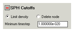
These options let you set SPH cutoffs.
The default values are usually good if you are using the default units (mm, mg, ms). You may want to change one or more of these defaults if you are using some other set of units.
Limit density / Delete node
If the density of an SPH node drops below the minimum density or above the maximum density defined by the minimum and maximum density factor chosen for the material, you have the choice of either limiting the density to the cutoff density or deleting the node. Make your choice here.
Minimum timestep
Nodes that have a timestep below the minimum timestep will be deleted.
Gravity
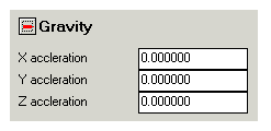
This option lets you set gravitational components for your model.
X / Y / Z acceleration
Enter the X Y and Z components of gravity in these fields.
The gravitational acceleration components will be applied to all Parts present in the model.
Transport
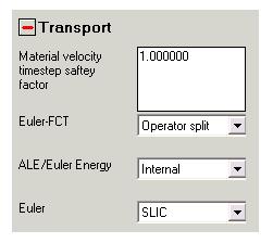
These options relate to the transport of material in various Solvers.
Material velocity timestep safety factor
Enter the timestep safety factor for material velocities.
In the velocity used to calculate the stability timestep is c+u, where c is the soundspeed of the material and u is its physical velocity.
If u is of the order of or greater than c, then using c + u/f can give more stable results, where f is the safety factor.
Euler-FCT
Select the type of transport algorithm that is used for Euler-FCT calculations from this pull-down menu. The default setting is multi-dimensional where all three spatial dimensions are solved simultaneously which is more efficient and helps to maintain symmetric flow fields. The alternative is Operator Split where each spatial dimension is solved in turn.
ALE/Euler Energy
During a computational Euler cycle mass, momentum and energy is being transported (fluxed) from element to element. This option determines if total energy or internal energy is being transported.
Total
This option conserves the total energy (kinetic + internal energy) during transport. This is the most robust and accurate option and is the default.
Internal
This option conserves the internal energy during transport. In cases where the total energy transport doesn't provide an accurate answer, e.g. material overheating or when the kinetic energy is predominant, the Internal option might be chosen as an alternative.
Euler
This option determines which transport algorithm will be used for multi-material transport.
SLIC
When material is being transported out of an element that contains multiple materials or voids, it is necessary to use special rules to determine the amount of each material being transported, because the only information available for the transport algorithm is the fraction of each material in the individual elements. In Autodyn the Simple Lime Interface Calculation (SLIC) method is used which uses a small number of stereotypes of mixed material element topologies. The SLIC algorithm is the default and works well for all multi-material Euler analysis.
Updated SLIC
Isolated small parts of material smaller than an element do not move through the mesh at the correct velocity. They tend to stop moving while surrounding material rushes by. The Updated SLIC option will transport these small material fractions with statistically the correct velocity. This option should be used with care, because it can have some undesirable side effects. It is possible for these small material fragments to "tunnel" through other multi-material Euler objects like walls or plates and emerge at the other side.
Global Erosion
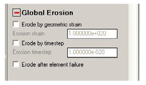
These options define global erosion criteria for all elements in the model. The global erosion options are only available for unstructured elements.