Start Ansys Polymat by typing polymat. Then follow the
procedure described below to perform the fitting for the data presented in Experimental Data.
Note: The fitting calculation for this example will take significant time, due to the transient elongational curves added for the fitting.
![]() Select Fluid Model
Select Fluid Model
Choose Differential viscoelastic model.
 Differential viscoelastic model
Return to the top-level menu.
![]() Material Data
Material Data
Enter the Differential viscoelastic models menu.
Differential viscoelastic models
Specify the first viscoelastic model.
1-st viscoelastic model
Select the Giesekus model.
Giesekus model
Accept the current values.
Accept current values
Return to the Differential viscoelastic models menu.
Upper level menu
Specify the second, third and fourth viscoelastics models of type
Giesekus.
Addition of a viscoelastic model
Note: You do not have to change values of the different modes. They will be fitted automatically later.
Return to the top-level Ansys Polymat menu.
Enter the Automatic Fitting menu.
Automatic fitting
Enter the List of Experimental Curves menu.
Add experimental curves
Add the first experimental curve (
visc.crv).
Add a new curve
Select the curve named visc.crv.
Enter the name of the curve file
Specify that the curve is a shear viscosity curve.
Modify the curve type
Choose steady shear viscosity (the default).
steady shear viscosity
Return to the List of Experimental Curves menu.
Add the second experimental curve (
g1.crv).
Add a new curve
Select the curve named g1.crv.
Enter the name of the curve file
Specify that the curve is a storage modulus curve.
Modify the curve type
Choose storage modulus G’.
storage modulus G’
Return to the List of Experimental Curves menu.
Add the third experimental curve (
g2.crv).
Add a new curve
Select the curve named g2.crv.
Enter the name of the curve file
Specify that the curve is a loss modulus curve.
Modify the curve type
Choose loss modulus G".
loss modulus G"
Return to the List of Experimental Curves menu.
Add the fourth experimental curve (
stress_01.crv).
Add a new curve
Select the curve named stress_01.crv.
Enter the name of the curve file
Specify that the curve is a transient extensional flow curve.
Modify the curve type
Choose transient extensional flow.
transient extensional flow
In this menu, choose uniaxial mode, stress vs. strain [ln(l/lo)], and constant extensional velocity.
In the menu Experimental curve #4, modify the initial strain rate (V/lo) and set it to
0.1.
Modify the initial strain rate
(V/lo)
Return to the List of Experimental Curves menu.
Add the fifth experimental curve (
stress_1.crv).
Add a new curve
Select the curve named stress_1.crv.
Enter the name of the curve file
Specify that the curve is a transient extensional flow curve.
Modify the curve type
Choose transient extensional flow.
transient extensional flow
In this menu, choose uniaxial mode, stress vs. strain [ln(l/lo)], and constant extensional velocity.
In the menu Experimental curve #5, modify the initial strain rate (V/lo) and set it to
1.
Modify the initial strain rate
(V/lo)
Return to the List of Experimental Curves menu.
Add the sixth experimental curve (
stress_10.crv).
Add a new curve
Select the curve named stress_10.crv.
Enter the name of the curve file
Specify that the curve is a transient extensional flow curve.
Modify the curve type
Choose transient extensional flow.
transient extensional flow
In this menu, choose uniaxial mode, stress vs. strain [ln(l/lo)], and constant extensional velocity.
In the menu Experimental curve #5, modify the initial strain rate (V/lo) and set it to
10.
Modify the initial strain rate
(V/lo)
Return to the List of Experimental Curves menu.
Return to the Automatic Fitting menu.
Plot the six experimental data curves.
Draw experimental curves
The curves will be presented in two graphics: In the first one, you can see the steady shear viscosity, G’ and G"; while in the second, you can see the extensional curves.
Set the numerical parameters for the calculation.
Numerical options for fitting
Limit the range of relaxation times to be from a minimum of
0.01to a maximum of100.
Modify the range of relaxation times
Return to the Automatic Fitting menu.
Specify a name for the material data file (for example,
example4.mat).
Enter the name of the result file
Start the fitting calculation.
Run fitting
The results of the fitting calculation are as follows:
RESULTS
nb. of modes = 4

 mode # 1 - Giesekus model
 T = T1 + T2
 (1+alfa*trelax/visc1*T1)*T1 + trelax*T1up = 2*visc1*D
 T2 = 2*visc2*D

 where - visc is the viscosity
       - visc1 = (1-ratio)*visc
       - visc2 = ratio*visc
       - trelax is the relaxation time
       - T1up is the upper-convected time derivative of T1

 visc   = 0.1940853E+04 [auto]
 trelax = 0.1000000E-01 [auto]
 alfa   = 0.7392697E+00 [auto]
 ratio  = 0.2350520E-04 [auto]

 mode # 2 - Giesekus model

 T = T1 + T2
 (1+alfa*trelax/visc1*T1)*T1 + trelax*T1up = 2*visc1*D
 T2 = 2*visc2*D

 where - visc is the viscosity
       - visc1 = (1-ratio)*visc
       - visc2 = ratio*visc
       - trelax is the relaxation time
       - T1up is the upper-convected time derivative of T1

 visc   = 0.1129548E+05 [auto]
 trelax = 0.2154435E+00 [auto]
 alfa   = 0.6407529E+00 [auto]
 ratio  = 0.0000000E+00 [fixed]

 mode # 3 - Giesekus model

 T = T1 + T2
 (1+alfa*trelax/visc1*T1)*T1 + trelax*T1up = 2*visc1*D
 T2 = 2*visc2*D

 where - visc is the viscosity
       - visc1 = (1-ratio)*visc
       - visc2 = ratio*visc
       - trelax is the relaxation time
       - T1up is the upper-convected time derivative of T1

 visc   = 0.4098902E+05 [auto]
 trelax = 0.4641589E+01 [auto]
 alfa   = 0.4906601E+00 [auto]
 ratio  = 0.0000000E+00 [fixed]

 mode # 4 - Giesekus model


 T = T1 + T2
 (1+alfa*trelax/visc1*T1)*T1 + trelax*T1up = 2*visc1*D
 T2 = 2*visc2*D

 where - visc is the viscosity
       - visc1 = (1-ratio)*visc
       - visc2 = ratio*visc
       - trelax is the relaxation time
       - T1up is the upper-convected time derivative of T1

 visc   = 0.4973851E+04 [auto]
 trelax = 0.1000000E+03 [auto]
 alfa   = 0.4113689E+00 [auto]
 ratio  = 0.0000000E+00 [fixed]
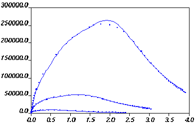
The computed and experimental curves are shown in Figure 10.4: Computed and Experimental Curves for Steady Shear Viscosity, Storage Modulus and Loss Modulus and Figure 10.5: Computed and Experimental Curves for Stress vs. ln(l/lo) at Different Initial Strain Rates (0.1,1, and 10)..
Figure 10.4: Computed and Experimental Curves for Steady Shear Viscosity, Storage Modulus and Loss Modulus
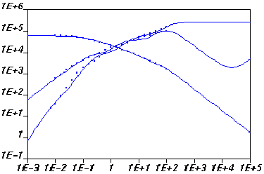
Figure 10.5: Computed and Experimental Curves for Stress vs. ln(l/lo) at Different Initial Strain Rates (0.1,1, and 10).