10.1.2. Fitting Procedure in Ansys Polymat

Start Ansys Polymat by typing polymat. Then follow the procedure below to perform the fitting for the data presented in Experimental Data.

10.1.2.1. Step 1: Define the Fluid Model Type

Select Fluid Model

Choose a Generalized Newtonian non-isothermal model.
Generalized Newtonian non-isothermal model
Return to the top-level menu.

10.1.2.2. Step 2: Specify the Material Data Models and Fix Parameters

Material Data

Specify the shear-rate dependence.
Shear-rate dependence of viscosity
1. Select the Carreau-Yasuda law.
  Carreau-Yasuda law
2. Return to the Material Data menu.
Specify the temperature dependence.
Temperature dependence of viscosity
1. Select the Arrhenius shear stress law.
  Arrhenius shear stress law
2. Enable the fixing of parameters.
  1. Click the Fix button at the top of the Ansys Polymat menu.
  2. Click OK to confirm that fixing is enabled.
3. Fix the value of to be 240.
  1. Specify .
    Modify talfa
  2. Specify that is fixed.
    talfa is a fixed value
  3. Return to the Arrhenius shear stress law menu.
4. Fix the value of to be .
  1. Specify .
    Modify t0
  2. Specify that is fixed.
    t0 is a fixed value
  3. Return to the Arrhenius shear stress law menu.
5. Disable the fixing of parameters.
  1. Click the Fix button at the top of the Ansys Polymat menu.
  2. Click OK to confirm that fixing is disabled.
6. Return to the top-level Ansys Polymat menu.

10.1.2.3. Step 3: Read in and Draw the Experimental Data Curves

Enter the Automatic Fitting menu.
Automatic fitting
Enter the List of Experimental Curves menu.
Add experimental curves
Add the first experimental curve (temp_200.crv).
Add a new curve
1. Select the curve named temp_200.crv.
  Enter the name of the curve file
2. Set the reference temperature to 200.
  Modify the temperature
3. Return to the List of Experimental Curves menu.
Add the second experimental curve (temp_220.crv).
Add a new curve
1. Select the curve named temp_220.crv.
  Enter the name of the curve file
2. Set the reference temperature to 220.
  Modify the temperature
3. Return to the List of Experimental Curves menu.
Repeat to add the third and fourth experimental curves (temp_240.crv and temp_260.crv) and set the appropriate reference temperatures.
Return to the Automatic Fitting menu.
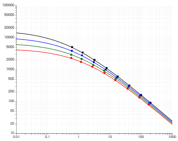
Plot the four experimental data curves.
Draw experimental curves

10.1.2.4. Step 4: Run the Fitting Calculation

Specify a name for the material data file (for example, example1.mat).
Enter the name of the result file
Start the fitting calculation.
Run fitting

10.1.2.5. Results

The results of the fitting calculation are as follows:

RESULTS

Carreau-Yasuda law

f(g) = facinf + (fac-facinf) *
[1+(tnat*g)**expoa]**((expo-1)/expoa)

fac      =  0.6793715E+04 [auto]
tnat     =  0.9776775E+00 [auto]
expo     =  0.1625742E+00 [auto]
facinf   =  0.9628369E-03 [auto]
expoa    =  0.5421551E+00 [auto]


Arrhenius shear stress law

h(t) = exp( alfa / (t-t0) - alfa / (talfa-t0) )

alfa     =  0.5559034E+04 [auto]
talfa    =  0.2400000E+03 [fixed]
t0       = -0.2731500E+03 [fixed]

The computed and experimental curves are shown in Figure 10.1: Plot of Computed and Experimental Curves.

Figure 10.1: Plot of Computed and Experimental Curves