


Ansys Polyflow provides options for decoupling the calculation of various fields, depending on the setup of the simulation.
A simulation that includes an Internal radiation sub-task is computationally expensive. For example, if a 3D domain is discretized into six radiative directions, the simulation will basically require as many variables as a single-mode viscoelastic model. Most of the time, at least 12 directions will be used to reach a reasonable accuracy. Internal radiation calculations are thus good candidates for decoupled schemes, with respect to the demands on both the CPU and memory.
The Numerical parameters menu offers the following three options for internal radiation problems. Note that the currently selected option is listed at the top of the menu.
a coupled calculation
For a coupled calculation, the velocities, irradiance, and temperature are all solved in the same pass. This is the default approach, and the most expensive from a computational and memory standpoint. If the setup has been changed from the default, you can enable a coupled calculation by selecting Coupled computation {velocities,irradiance,temperature} (note that this option is not available until you have already clicked Decoupled computation velocities/irradiance/temperature).
 Coupled computation
{velocities,irradiance,temperature}
Coupled computation
{velocities,irradiance,temperature}
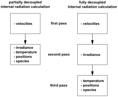
a partially decoupled calculation
For a partially decoupled calculation, the momentum equation is solved in a first pass, and then the irradiance and temperature are solved in a second pass. It is often a good choice, because irradiance and temperature are coupled. To enable a decoupled, two-pass calculation, click Decoupled computation velocities/{irradiance,temperature} (note that this option is not available until you have already clicked Coupled computation {velocities,irradiance,temperature}).
Decoupled computation
velocities/{irradiance,temperature}
a fully decoupled calculation
For a fully decoupled calculation, the momentum equation is solved in a first pass, then the irradiance is solved in a second pass, and finally temperature is solved in a third pass. Such a calculation yields iterations that are the most inexpensive from a computational and memory standpoint, but it might require more iterations. It is a good choice when your computer memory is limited. To enable a decoupled, three-pass calculation, click Decoupled computation velocities/irradiance/temperature (note that this option is not available until you have already clicked Decoupled computation velocities/{irradiance,temperature}).
Decoupled computation
velocities/irradiance/temperature
When solving moving boundary problems, you can decouple the calculation of the flow field from the node position update. This scheme will exhibit increased numerical stability in some cases. To use this scheme, select Decoupled computation of moving surfaces in the Numerical parameters menu.
Although it requires more total CPU time than the coupled approach in most cases, the decoupled approach is of interest in a number of applications. In blow molding applications, since the time steps are usually limited by the contact detection algorithm, decoupling can actually result in a significant speedup in the total CPU time.
When the position update is decoupled from the velocity calculation, the computations are made first with an update of the positions, followed by iterations to solve the velocity-pressure-temperature-etc. problem, then back to compute the next position update. The main application of decoupled free surfaces is related to integral viscoelastic models and blow molding applications (see Additional Strategies for Convergence).
When a simulation with a Transport of species sub-task is defined, Ansys Polyflow needs to compute a species concentration field in addition to the velocity, pressure, and possibly other fields such as temperature, position, and stresses. By default, Ansys Polyflow solves for all of the variables at the same time. In an attempt to reduce the demands on the CPU and memory, you can decouple the computation of the transported variable from the other fields. To enable this scheme, click Decoupled computation velocities/species in the Numerical parameters menu.
![]() Decoupled computation velocities/species
Decoupled computation velocities/species
When you enable this decoupling, the equations are solved in two stages. First, the mass and momentum (and possibly position) equations are solved, considering the species concentration as given. Either the concentration calculated at the previous iteration or the initial concentration is used. Then, the transport equation is solved alone, considering other equations as given. These two stages are repeated until all of the variables have converged. The mass and momentum equations are solved first because the velocities contribute to the transport equation.
The advantage of this technique is the reduction of both memory requirements and CPU time per iteration. The disadvantage is the possibly lower rate of convergence with respect to a fully coupled solver when a strong coupling exists between the momentum and transport equations. In rare cases, the decoupled technique can result in divergence, even though the coupled solver converges. For 2D problems, it is recommended that you always use the coupled technique, because the reduction of CPU time with decoupling will not be significant.
When a nonisothermal flow problem is defined, Ansys Polyflow needs to compute a temperature field in addition to velocity, pressure, and possibly other fields such as position and stresses. Because the Prandtl number of most polymers is large, the Péclet number of the flow can be high and a refined interpolation might be required for the temperature field, such as the combination of the linear interpolation for velocity and the subdivided 2×2×2 temperature element in 3D.
By default, Ansys Polyflow solves for all variables at the same time. In an attempt to reduce the memory and CPU time for a subset of nonisothermal problems, you can decouple the computation of the velocity-pressure variables from the temperature calculation. To use this scheme, select Decoupled computation velocities/temperature in the Numerical parameters menu.
When you select this decoupling, the equations are solved in two stages. First, the mass and momentum (and possibly position) equations are solved considering the temperature as given. Either the temperature calculated at the previous iteration or the initial temperature is used. Then, the energy equation is solved alone, considering other equations as given. These two stages are repeated until all variables have converged. The mass and momentum equations are solved first because the velocities contribute to the convective and viscous dissipation terms in the energy equation. If the simulation includes contact detection, like blow molding or thermoforming, the convection and the viscous heating effects are not dominant in the equations. Thus, the sequence of decoupling is reversed: the energy equation is computed first, and then the velocity and pressure are computed.
The advantage of this technique is the reduction of both memory requirements and CPU time per iteration. The disadvantage is the possibly lower rate of convergence with respect to a fully coupled solver when a strong coupling exists between the momentum and energy equations. The typical case where the technique is useful is when the viscosity of the fluid is independent of the temperature or only slightly dependent, and when natural convection (Boussinesq terms) is neglected. In this case, momentum and continuity equations together, and the energy equation on its own, can be solved one after the other, and the convergence rate is the same as for the coupled technique.
However, when natural convection dominates in the momentum equation, when the temperature strongly influences the viscosity (which is the case for many polymers), neglecting cross momentum-energy derivatives may reduce the rate of convergence. This can result in an increase in the CPU time because the number of iterations may increase more quickly than the CPU time per iteration decreases. In rare cases, the decoupled technique can result in divergence even though the coupled solver converges.
For example, for an Arrhenius law, use the decoupling technique with care if the energy of activation is higher than 3000 and when you expect temperature differences on the order of 30°C or more in the flow. For 2D problems, always use the coupled technique because the reduction of CPU time with decoupling will not be significant.
Important: A dependence of the temperature upon the velocity, through the advection or viscous dissipation terms, for example, will not affect the rate of convergence. Even in the case when the Péclet number is high, the advection term itself will not degrade convergence (but it might affect the solution accuracy if the mesh is not sufficiently fine).
When a viscoelastic flow problem is defined, Ansys Polyflow needs to compute several additional tensor variables (stress, configuration, orientation, rate of deformation) in addition to velocity, pressure, and possibly other fields such as position, species, or temperature. These tensor variables contribute to a substantial increase of the number of unknowns, and it is not unusual that the total number of unknowns be several times larger than that of a corresponding inelastic Newtonian flow with identical discretization.
Because of the relatively large number of unknowns and their increased connectivity that are typical of viscoelastic flow simulations, the solver may require computational resources (memory) beyond the availability on the computer. By default, viscoelastic variables are solved together with velocity, pressure and other unknowns, as this is shown to exhibit the best performances. However, when the memory requirement for a simulation reaches the computer limits, you should consider decoupling the calculation of viscoelastic variables from the other unknowns. This can be accomplished by selecting Decoupled computation of viscoelastic stresses in the Numerical parameters menu:
![]() Decoupled computation of viscoelastic stresses
Decoupled computation of viscoelastic stresses
Considering temperature, for example, when you select this decoupling, the equations are solved in two sequences. First, the mass and momentum (and possibly position) equations are solved considering the viscoelastic variables as given from the previous iteration. Then, the constitutive equations are solved alone, considering other fields as given. These two sequences are repeated until all variables have converged. The mass and momentum equations are solved first because the fluid flow is at first dictated by boundary conditions given in terms of velocity and/or force.
The primary motivation of a decoupled calculation of viscoelastic stresses is the substantial reduction of memory requirement that can be expected. However, there may have some drawbacks: the calculation time may increase because the convergence rate is slowed down, and usually lower values of the Weissenberg number can be reached.
Decoupled calculation of viscoelastic stresses can be activated for 2D and 3D flows, steady and transient flows, isothermal and non-isothermal flows. It is also probably the only viable option for large multi-mode viscoelastic flows. It is not, however, applicable for the Leonov model, and it is available only when the EVSS, EVSS-SU, DEVSS or DEVSS-SU methods are invoked.
If you decouple the calculations for temperature, viscoelastic stresses, moving boundary, and species, three sequences will be created: velocity and pressure will be computed together, temperature, species and positions will be solved in a second sequence, while viscoelastic stresses will be solved in the last sequence.
In the case of a setup with internal radiation, irradiance is always computed in the second pass. The temperature, positions, and/or species are always computed in the last pass of the calculation, which may be the second pass or the third pass, depending on the selected strategy for radiation. See Figure 31.1: Field Calculation Order for Internal Radiation for further details.
For all non-isothermal simulations, with the exception of elasticity and radiation, you have the option of setting the Operating temperature in the Numerical parameters menu. Using this menu, you can set the operating temperature to one of three modes:
Select mode: temperature computed (the default) - this mode allows you to have the temperature field calculated using the energy equation according to the initial temperature (defined in the average temperature menu or read in a RES or CSV file), heat sources, and the boundary conditions.
Select mode: temperature frozen - this mode allows you to keep the initial temperature (defined in the average temperature menu or read in a RES or CSV file) unchanged during the entire calculation. Temperature dependent parameters are evaluated at the local temperature.
Select mode: process temperature imposed - this mode allows you to define a constant temperature on the whole calculation domain, where that temperature will be kept constant during the computation. Temperature dependent parameters are evaluated at the specified process temperature.
The setup is slightly adapted when the operating mode is set to Select mode: temperature frozen or Select mode: process temperature imposed. The convergence strategy for thermal flows and/or decoupled computation of velocities/temperature are/is disabled. Temperature boundary conditions are not taken into account during resolution.
The Select mode: temperature frozen and Select mode: process temperature imposed modes allow you to perform impossible experiments, to reduce the calculation time, or to accelerate convergence when thermal effects are moderate and an approximate solution is valuable, or to facilitate the setup of isothermal calculations at precise temperatures using temperature-dependent material data that will be correctly evaluated at the process temperature.