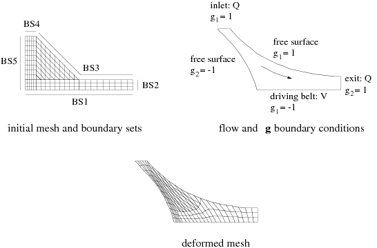
Consider the example shown in Figure 16.4: Coating Example for Thompson Transformation. This flow problem models a coating process, which involves two free surfaces. A Thompson transformation is used for the whole domain, since large mesh deformations are expected. The boundary conditions are described as follows: the fluid enters the flow domain at the top, is driven at the bottom by a belt that moves from left to right, and exits the computational domain on the right-hand side; the two remaining sides are free surfaces.
Five boundary sets are defined in Figure 16.4: Coating Example for Thompson Transformation,
and boundary conditions are selected so that the mesh domain maps logically onto a
square (2D) or cube (3D) region. The choice of  or
or  is not always unique. Values on opposite sides of the square or
cube must be different, but the value itself is not relevant. For this reason,
values of 1 and
is not always unique. Values on opposite sides of the square or
cube must be different, but the value itself is not relevant. For this reason,
values of 1 and  are generally used. On BS1, a value of
  for
for  is imposed. On BS3 and BS4,
  ; on BS2,
  ; and on BS5,
  . In general, a zero-normal-derivative condition is imposed on
boundary sets without an imposed component, in order to close the problem. A
zero-normal-derivative condition is therefore imposed for
. In general, a zero-normal-derivative condition is imposed on
boundary sets without an imposed component, in order to close the problem. A
zero-normal-derivative condition is therefore imposed for  on BS2 and BS5, and for
  on BS1, BS3, and BS4. Ansys Polyflow will calculate the solution of
the Laplace equation for both
on BS1, BS3, and BS4. Ansys Polyflow will calculate the solution of
the Laplace equation for both  and
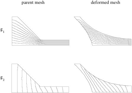
and  . This solution is shown in Figure 16.5: The g Field for the Thompson Transformation.
Then, upon deformation of the mesh, Ansys Polyflow will relocate nodes in such a way
that
. This solution is shown in Figure 16.5: The g Field for the Thompson Transformation.
Then, upon deformation of the mesh, Ansys Polyflow will relocate nodes in such a way
that  and
and  are unchanged for a given node. Contour lines of the
 and
and  fields are shown on the deformed and original (parent) meshes in
Figure 16.5: The g Field for the Thompson Transformation. The corresponding mesh is shown in Figure 16.4: Coating Example for Thompson Transformation.
fields are shown on the deformed and original (parent) meshes in
Figure 16.5: The g Field for the Thompson Transformation. The corresponding mesh is shown in Figure 16.4: Coating Example for Thompson Transformation.