


The Navier-Stokes equations are modified to become
 | (22–1) |
| where |

| is a step function |

| is the velocity | |

| is the local velocity of the moving part | |

| is the pressure | |

| is the extra-stress tensor | |

| is the volume force | |

| is the acceleration term |
For a generalized Newtonian fluid, the extra-stress tensor is defined to be
 | (22–2) |
| where |

| is the viscosity |

| is the shear rate | |

| is the temperature | |

| is the rate-of-deformation tensor |
Equation 22–1 is then
discretized for each node of the velocity field. For node  (at location
  ), if it is outside the moving part, then
  is equal to 0 and the usual Navier-Stokes equations are used.
Otherwise,
is equal to 0 and the usual Navier-Stokes equations are used.
Otherwise,  is set to
  , and Equation 22–1 degenerates into
 | (22–3) |
in order to impose the local velocity  of the moving part.
More specifically, before solving the Navier-Stokes equations, the "inside" field
 is calculated for the flow domain. This field varies between 0 and
1. A subelement that is overlapped by the moving part has a value of
is calculated for the flow domain. This field varies between 0 and
1. A subelement that is overlapped by the moving part has a value of  , and a subelement outside the moving part has a value of
 . A node
  (at location
  ) is considered to be inside the moving part (that is,
 ) if
) if  is greater than a threshold value. The threshold value is usually
equal to 0.6, which indicates that more than half of the subelements neighboring the
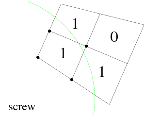
node are overlapped by the moving part. Figure 22.2: “Inside" Field for a 2D Finite Element shows a 2D finite element divided into 4 subelements. The
subelements that are overlapped by the moving part are marked with a 1, and those
that are outside the moving part are marked with a 0. The nodes for which
is greater than a threshold value. The threshold value is usually
equal to 0.6, which indicates that more than half of the subelements neighboring the
node are overlapped by the moving part. Figure 22.2: “Inside" Field for a 2D Finite Element shows a 2D finite element divided into 4 subelements. The
subelements that are overlapped by the moving part are marked with a 1, and those
that are outside the moving part are marked with a 0. The nodes for which
 are indicated by filled-in circles.
The previous explanation of the Navier-Stokes equation assumes a full stick condition along the borders of the moving part. You have the option of enabling a slip condition along the borders of the moving part. Note that because the moving part is represented by means of a domain that overlaps the fluid region (as explained previously), the fluid region will experience only an approximation of the actual boundary of the solid moving part. Because of this approximation, the slipping will be handled by bounding the local value of the shear stress (by a value you specify). In other words, the slipping behavior will obey a mechanism that resembles the asymptotic law given by Equation 8–3. More precisely, if the local value of the shear stress is below the value you specify, the material will be treated as if it is sticking to the wall of the moving part; otherwise, the maximum slipping stress will be applied.