


The inputs for 2D and 3D models that are directly related to the contact detection are provided in this section. See Inputs for Shell Contact Detection for information about setting up contact detection for a shell model. You can set up the rest of the problem (material properties, other boundary conditions, and so on) as usual. See Remeshing for information about remeshing.
Create a task of the time-dependent type.
 Create a new task
Define the mold(s).
Define molds
Create a mold.
Create a new mold
Specify the type of mold. There are three options:
To model an adiabatic mold, select Adiabatic mold:
Adiabatic mold
If you select this option, there will be no heat exchange between the mold and the fluid in contact.
To model a mold that remains at a constant specified temperature throughout, select Mold with constant and uniform temperature:
Mold with constant and uniform
temperature
If you select this option, the heat transfer between the mold and the fluid in contact will be taken into account in the calculation. The heat transfer is governed by a heat transfer coefficient and a mold temperature.
To model conjugate heat transfer between the mold and the fluid, select Mold with temperature calculation:
Mold with temperature calculation
If you select this option, Ansys Polydata will disable the option to use shell elements for the parison. This is because shell elements cannot be used in a simulation that involves conjugate heat transfer between the parison and the mold.
When prompted, specify a name for the mold.
Specify the region (subdomain or subdomains) that represents the mold.
Domain of the mold
If a mold is composed of several subdomains, which are assigned the same motion, define these subdomains as the domain of the mold.
If you selected the Mold with temperature calculation option, define the density, thermal conductivity, heat capacity per unit mass, average temperature, and heat source per unit volume.
Material data
See Problem Setup for details about specifying these thermal properties. The average temperature that you specify applies only to this particular mold, and serves as an initial temperature condition.
If you selected the Mold with temperature calculation option, define the thermal boundary conditions for it.
Thermal boundary conditions
See Problem Setup for details about specifying thermal boundary conditions. Note that the wall along which contact has been defined will be considered insulated until contact occurs.
Specify which boundary represents the part of the mold that comes into contact with the fluid. When a point of a free surface enters a solid mold, Ansys Polyflow computes the penetration length. This length is the distance between the point and the boundary of the solid mold or contact domain. Usually, it is efficient to restrict the contact domain boundary to the part that the free surface actually touches. Hence, it is recommended that the boundary of the mold be defined by different boundary sets. In this step, you choose which part must be taken into account to compute the penetration length.
Contact conditions
Select the boundary that is in contact with the free surface and click Modify.
Select Contact in the resulting menu and then select Upper level menu.
Repeat if there are other boundaries that contact the free surface.
Select Upper level menu again to continue the mold definition.
Specify the motion of the mold, if required.
Mold motion
When you select Mold motion, the selected attributes are displayed.
Specify the mold motion, if required:
Modify motion type: fixed mold
Enter a New value in the Specify the type of mold motion dialog box that opens to indicate the motion type of the mold:
Enter
0to fix the mold (that is, no velocity or force imposed).Enter
1to impose a translation velocity.Enter
2to impose a translation force.Enter
3to impose a general velocity driven motion.
Click to close the Specify the type of mold motion dialog box.
If you opted to impose a translation velocity on the mold, define the velocity.
Select Modify translation velocity:
Modify translation velocity
When prompted, enter the value of the translation velocity in each coordinate direction.
Select Modify angular velocity to specify the angular velocity for the solid mold:
Modify angular velocity
This option is available only for 2.5D axisymmetric problems. The rotation axis is always the Z axis.
If you opted to impose a translation force on the mold, define the settings.
Select Modify translation force:
Modify translation force
When prompted, enter the value of the translation force in each coordinate direction.
Select Modify initial velocity to specify the initial velocity, if required:
Modify initial velocity
When prompted, enter the value of the initial velocity in each coordinate direction.
Specify the mass of the mold:
Modify mass of mold
This value corresponds to the total mass of the mold and of the moving part connected to the mold.
Specify the maximum mold displacement:
Modify max displacement
This value corresponds to the maximum admissible displacement along the direction specified by the force. The mold motion will continue until either the maximum displacement is reached, the specified time duration is reached, or the solution diverges.
For shell models, the maximum displacement must be bounded, and hence this quantity is uninitialized when you open the menu for the first time. Subsequently, the maximum displacement can be modified.
For models other than shell models, you may decide whether the mold displacement must be bounded and to what value.
If you opted to impose a general velocity to the mold, define the settings. The description of the general motion is similar to that applied for the motion of moving parts (see Description of Motion).
Select Modify the point of local rotation axis:
Modify the point of local rotation
axis
When prompted, enter the coordinates of the point of the local rotation axis.
Select Modify the orientation of local rotation axis:
Modify the orientation of local rotation
axis
When prompted, enter the vector components of the orientation of the local rotation axis. Note that for 2D flows, the rotation axis is perpendicular to the XY plane.
Select Modify the angular velocity:
Modify the angular velocity
When prompted, enter the value for the angular velocity. Note that the angular velocity must be given in revolutions per second (or rps).
Select Modify the translation velocity:
Modify the translation velocity
When prompted, enter the components of the translation velocity applied to the rotation axis. Note that evolution functions can be applied to the translation velocity.
Select Modify the initial angle of rotation:
Modify the initial angle of
rotation
When prompted, enter the value for an initial orientation to the mold. Note that the initial angle of rotation must be given in degrees.
Select Modify the initial translation vector:
Modify the initial translation
vector
When prompted, enter the components of the translation vector applied for modifying the initial position to the rotation axis of the mold.
Select Modify the initial theta angle (Z axis) to change the initial direction of the axis of rotation by an angle
 around the Z-axis.
Modify the initial theta angle (Z
axis)
around the Z-axis.
Modify the initial theta angle (Z
axis)
When prompted, enter the value for the angle
. This parameter is available only
for shell and 3D models. Note that the theta angle
must be given in degrees. Select Modify the initial phi angle (Y axis) to change the initial direction of the axis of rotation by an angle
 around the new Y-axis subsequent
to the change under the previous step (G).
Modify the initial phi angle (Y
axis)
around the new Y-axis subsequent
to the change under the previous step (G).
Modify the initial phi angle (Y
axis)
When prompted, enter the value for the angle
. This parameter is available only
for shell and 3D models. Note that the phi angle
must be given in degrees.Select Modify the angular velocity Vtheta (Z axis) to specify the angular velocity of the rotation axis around the Z-axis.
Modify the angular velocity Vtheta (Z
axis)
When prompted, enter the value for the angular velocity Vtheta. This parameter is available only for shell and 3D models. Note that the angular velocity Vtheta must be given in revolution per second (or rps).
Select Modify the angular velocity Vphi (Y axis) to specify the angular velocity of the rotation axis around the new Y-axis subsequent to the change under the previous step (I).
Modify the angular velocity Vphi (Y
axis)
When prompted, enter the value for the angular velocity Vphi. This parameter is available only for shell and 3D models. Note that the angular velocity Vphi must be given in revolution per second (or rps).
Select Upper level menu repeatedly to return to the Define molds menu, where you can repeat the steps above to define another mold, if necessary.
Select Upper level menu to return to the task menu where you will continue the problem setup.
Create a sub-task of the appropriate type for the fluid:
Generalized Newtonian isothermal flow problem
Generalized Newtonian non-isothermal flow problem
Differential viscoelastic isothermal flow problem
Differential viscoelastic non-isothermal flow problem
Specify the region where the sub-task applies.
Domain of the sub-task
Specify which boundary is the free surface.
In the Flow boundary conditions menu, select the boundary set that represents the free surface and click Modify.
Flow boundary conditions
Select Free surface as the boundary type.
Free surface
Define the free surface boundary conditions, following the procedure outlined in General Procedure.
Specify the contact detection problem.
Contact (Blow mold.)
Create a new contact problem.
Create a new contact problem
Specify where the free surface will contact the mold.
Select a contact wall
Select the appropriate contact wall (that is, the one you previously defined in the Define molds menu).
Click Select.
If you defined the mold as a Mold with constant and uniform temperature or a Mold with temperature calculation, specify the parameters for the heat flux across the contact boundary:
If the mold is at a constant temperature, specify the values for
 and
and  in Equation 17–5.
Modify alpha
in Equation 17–5.
Modify alpha
The default value for
is set to 1000. Since it is unit
dependent, it is advised to specify a more appropriate value
if necessary.
Modify T_mold
 will be the constant temperature of the
mold in this case.
will be the constant temperature of the
mold in this case. If you select the Mold with temperature calculation option (that is, if you are modeling conjugate heat transfer, described in Heat Transfer and Contact (Conjugate Heat Transfer)), specify the value for
 . You will not specify
  because the temperature of the mold is not
constant; it is computed by Ansys Polyflow during the
simulation.
because the temperature of the mold is not
constant; it is computed by Ansys Polyflow during the
simulation.
Enable contact release and define the adhesion force density (
 in Equation 17–3), if necessary.
Modify adhesion force density
in Equation 17–3), if necessary.
Modify adhesion force density
Contact release is disabled by default, as indicated by the description of the adhesion force density as being undefined in the Modify adhesion force density menu item. When you click this menu item, Ansys Polydata will ask you to confirm the enabling of contact release and then allow you to specify the New value for the adhesion force density. If you do not have test results or specifications to guide your definition of the adhesion force density, it is reasonable to start by replacing the default value of 0 with a small value in your unit system (for example, 10–100 Pa).
When you enable contact release, you must make sure that the slipping and penalty coefficients you define in step 7.e. and f. are set to the same value, so that slip at contact is not permitted. You should also enter low values for the penetration accuracy and element dilatation in step 7.g. and h., to allow the material to escape from the contact condition; this is especially important when the time steps are small. The goal is to have the penetration accuracy be smaller than the product of the velocity and the time step, though this can be difficult since low values of penetration accuracy result in small time steps. Finally, it is recommended that you set the convergence test value to 10-4 when you define the Numerical parameters in step 9. (see Convergence and Divergence for details).
Modify the slip coefficient (
 in Equation 17–2), if necessary.
Modify slipping coefficient
in Equation 17–2), if necessary.
Modify slipping coefficient
The default value is 1012. If the slip coefficient and the penalty coefficient have the same value, then it is assumed that the fluid sticks to the mold when it comes into contact. Full slippage at the contact boundary is assumed if the slip coefficient is zero. Actual cases involving partial slippage will require a slip coefficient that typically ranges from 102 to 106, depending on the physics involved as well as on the system of units being used.
Modify the penalty coefficient (
 in Equation 17–1), if necessary.
Modify penalty coefficient
in Equation 17–1), if necessary.
Modify penalty coefficient
The default value of 1012 is acceptable for most cases.
Modify the penetration accuracy, if necessary.
Modify penetration accuracy
If the penetration of a point into the mold is greater than the penetration accuracy, the time step will be rejected. The calculation will then be restarted from the previous time step with a smaller time-step increment. The default value is set according to the dimensions of the mesh, and you will generally not need to modify it.
Specify the element dilatation, if necessary.
Modify element dilatation
This option allows for expansion of each finite element of the mold in order to help the contact detection algorithm. Some numerical errors can cause a point to "miss" the mold. A typical case can occur when a point of the fluid domain is supposed to come into contact with a mold at the location of the symmetry line of the mold. A small expansion of the finite elements fixes the problem. The default value is set according to the penetration accuracy, and you will generally not need to modify it.
Select Upper level menu to return to the Define contacts menu, where you can repeat the steps above to define another contact wall for the free surface.
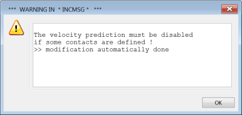
Select Upper level menu two times to complete the free surface and contact problem definition and return to the Flow boundary conditions panel. Ansys Polydata will warn you that the velocity prediction has been disabled. In contact detection problems, abrupt changes in the velocity field occur at the contact points between the fluid parison and the solid mold. These discontinuities prevent the prediction scheme from working properly, so it is automatically disabled for you. Click to continue.
Define the remeshing procedure for the sub-task (after you finish setting all boundary conditions and return to the sub-task menu one level above the Flow boundary conditions menu).
Global remeshing
See Remeshing for details.
Define the numerical parameters for the time-dependent task (one level above the sub-task menu).
Numerical parameters
See User Inputs for Time-Dependent Problems for details about the inputs for time-dependent calculations. If you select Modify the transient iterative parameters, you will see that the velocity field prediction has been disabled for you, as mentioned above. You should not reenable the velocity prediction for a contact detection problem.