In extrusion, blow molding, and injection stretch blow molding (ISBM) applications, extension evaluation is simple. Unit vector deformations are tracked based on the initially selected two natural directions with respect to the parison or preform axis—the axial and hoop directions. Depending on the requirements, one or two sets of vectors tangent to the shell are defined in a plane parallel and perpendicular to the axis. The first set involves vectors defined in planes containing the axis and the second set involves vectors orthogonal to the axis. Two such vectors are shown in Figure 17.4: Definition of Initial Vectors and Evaluation of Extension Along Directions Parallel and Perpendicular to the Axis of a Parison.

In thermoforming applications the initial sheet is often flat, hence vectors sets can initially be defined either as parallel and perpendicular to a given direction D or as radial and circumferential distributions around a point P. It is the process and the individual geometry that will dictate the choice.

Figure 17.4: Definition of Initial Vectors and Evaluation of Extension Along Directions Parallel and Perpendicular to the Axis of a Parison

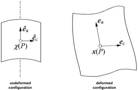
Consider a grid on the undeformed parison. At a point on this grid, two unit vectors, and are defined along a direction parallel and perpendicular to the axis, respectively. During inflation, the length and orientation of these vectors are affected, and these changes will record the resulting deformations. In particular, their magnitudes will provide quantitative information along both reference directions.

Consider an arbitrary fluid particle initially located at . At the end of the inflation step, is located at . In the vicinity of , the tensor of deformation gradients is given by

(17–15)

From there, the extension components ( and ) are evaluated from

(17–16)

and the magnitude of the extension components is given by the amplitudes and , respectively.

In addition to the extension components, which indicate the possible anisotropy of the deformations, it is also relevant to evaluate the area stretch ratio. A first approximation can be obtained by considering a material surface and calculating the ratio of its area in the deformed configuration to that in the undeformed state. Such a representation is easy, but not continuous.

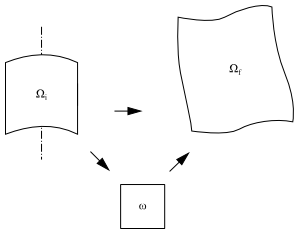
Ansys Polyflow uses a continuous representation that takes advantage of the finite-element technique and Lagrangian formulation. Internally, the numerical integration of the equations on a finite element requires a geometric transformation between the actual element and its parent element , as illustrated in Figure 17.5: Geometric Transformations for Evaluating the Area Stretch Ratio.

Figure 17.5: Geometric Transformations for Evaluating the Area Stretch Ratio

The transformation is based on a Jacobian . This Jacobian can be understood as the ratio of infinitesimal areas respectively considered in the actual and parent elements:

(17–17)

Consider the material element in its initial (undeformed) and final (deformed) configurations, and , respectively. For these configurations, the respective Jacobians are obtained from

(17–18)

From Equation 17–18, the area stretch ratio is given by

(17–19)

With a bilinear interpolation, nodal values for can be evaluated in a post-calculation based on the least mean squares technique. Hence, a continuous representation is obtained for .