


Whenever the boundary of a mesh undergoes significant displacement (for example, due to the deformation of the fluid region during parameterization or optimization of the geometry), the mesh must be adjusted to accommodate the new configuration. When adjustments are made using elastic remeshing, Ansys Polyflow treats the mesh as a pseudo-elastostatic medium and employs the same general algorithm that is used to calculate the displacement of an elastic solid. The mesh boundary conditions differ from those for the solid, however, in that only displacement boundary conditions are allowed, because boundary conditions that involve stresses or forces proportional to displacement have no meaning in the context of the mesh.
A potential drawback of modeling the mesh as an elastostatic medium is that the solver does not guarantee the production of a mesh in which element distortion is absent. In most practical applications, the mesh is not uniform and contains elements that are skewed, have high aspect ratios, or otherwise have bad quality. A straightforward treatment of the mesh as an isotropic homogeneous pseudo-elastic medium tends to distort all of elements in the same way, including the "bad" ones. In order to control mesh distortion due to remeshing, it is preferable to manipulate the pseudo-material elasticity matrix in such a way as to increase the stiffness of bad elements or elements whose quality is worsening. The major advantage of such an approach is that it can be done efficiently and is physically based.
In order to understand how the Ansys Polyflow elastic remeshing algorithm can
control mesh distortion, it is necessary to examine how the mesh quality and new
nodal positions are calculated. Consider an example where element 1 is made up of
nodes h, i, j, and k. A quality indicator ( ) for node i of element 1 is calculated using the following
equation:
) for node i of element 1 is calculated using the following
equation:
 | (35–5) |
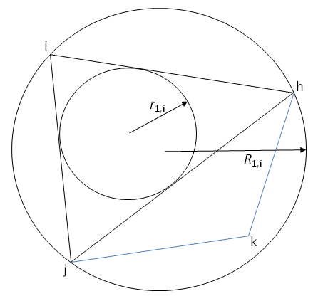
In the previous equation,  and
and  are radii of the circumcircle and the incircle, respectively, of a
triangle whose points include node i and the two nodes attached to i by a single
face in element 1 (that is, nodes h and j), as shown in Figure 35.2: The Circumcircle and Incircle for Node i on Element 1.
are radii of the circumcircle and the incircle, respectively, of a
triangle whose points include node i and the two nodes attached to i by a single
face in element 1 (that is, nodes h and j), as shown in Figure 35.2: The Circumcircle and Incircle for Node i on Element 1.
Note that the minimum value  can be is 2, which would be achieved if triangle h-i-j was
equilateral. Equation 35–5 gives
a large value for very thin elements (even if the element is a rectangle), or for
elements that have an angle close to 0 or
can be is 2, which would be achieved if triangle h-i-j was
equilateral. Equation 35–5 gives
a large value for very thin elements (even if the element is a rectangle), or for
elements that have an angle close to 0 or  . Table 35.1:
 as a Function of Height (
 ) shows
how the value of
) shows
how the value of  changes with height (
 ), if triangle h-i-j were one of the triangles illustrated in Figure 35.3: Height h for Two Kinds of Triangles.
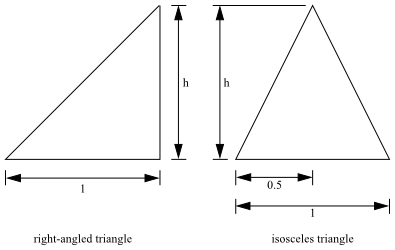
Table 35.1:
as a Function of Height ()

|

| |
| Right-Angled Triangle | Isosceles Triangle | |
| 100 | 100.5 | 100.5 |
| 10 | 10.6 | 10.5 |
| 5 | 5.7 | 5.6 |
| 2 | 2.9 | 2.7 |
| 1 | 2.4 | 2.0 |
| 0.5 | 2.9 | 2.4 |
| 0.2 | 5.7 | 7.5 |
| 0.1 | 10.6 | 26.3 |
| 0.01 | 100.5 | 2,501.3 |
| 0.001 | 1,000.5 | 250,001.3 |
While Figure 35.2: The Circumcircle and Incircle for Node i on Element 1 only shows
how  and
and  are defined for a 2D element, these variables can be also be
defined for a 3D element. For a 3D element,
are defined for a 2D element, these variables can be also be
defined for a 3D element. For a 3D element,  and
and  are radii of the circumsphere and insphere, respectively, of a
tetrahedron, whose points include a given node and the three nodes of an element
that are attached to it by a single edge.
are radii of the circumsphere and insphere, respectively, of a
tetrahedron, whose points include a given node and the three nodes of an element
that are attached to it by a single edge.
After the quality indicator is calculated at node i for element 1, the same
process is repeated for all of the other elements that share node i. A total quality
indicator for node i ( ) is then calculated by summing all of these values:
 | (35–6) |
where  represents the element index of every element that shares node i.
After the total quality indicators have been calculated for each node of the mesh,
these values are linearly interpolated in order to simultaneously calculate a field
of element quality indicators ( ) and the new nodal positions. The quality indicators and nodal
positions are recalculated during every iteration of the solution.
) and the new nodal positions. The quality indicators and nodal
positions are recalculated during every iteration of the solution.
The relationship between  and the new nodal positions depends on your setup parameters. As
stated previously, the elastic remeshing scheme is governed by the pseudo-elastic
equation (Equation 35–3), which includes
a variable that functions as Young’s modulus (
and the new nodal positions depends on your setup parameters. As
stated previously, the elastic remeshing scheme is governed by the pseudo-elastic
equation (Equation 35–3), which includes
a variable that functions as Young’s modulus ( ). Your setup can result in
  behaving like one of the following:
a function of the current and initial fields of element quality indicators

(35–7)
where
 is the initial field of element quality indicators
(calculated prior to any deformation) and
is the initial field of element quality indicators
(calculated prior to any deformation) and  is a user constant that is set to 2 by default. With this
equation, all elements have the same stiffness (that is,
is a user constant that is set to 2 by default. With this
equation, all elements have the same stiffness (that is,  ) for the first iteration. As the solution iterates, the
stiffness of each element will increase as it becomes more distorted
relative to its initial state, while the stiffness will decrease as it
becomes less distorted relative to its initial state. Note that Equation 35–7 is the
default definition for
) for the first iteration. As the solution iterates, the
stiffness of each element will increase as it becomes more distorted
relative to its initial state, while the stiffness will decrease as it
becomes less distorted relative to its initial state. Note that Equation 35–7 is the
default definition for  .
. a function of the current field of element quality indicators

(35–8)
where
 is a user constant that is set to 2 by default. With this
equation, the elements that have a worse quality indicator for a given
iteration are stiffer than those whose quality indicator is better.
Therefore, the good elements will be deformed more than the bad elements
during remeshing, immediately during the first iteration of the solution.
is a user constant that is set to 2 by default. With this
equation, the elements that have a worse quality indicator for a given
iteration are stiffer than those whose quality indicator is better.
Therefore, the good elements will be deformed more than the bad elements
during remeshing, immediately during the first iteration of the solution.
a unit value

(35–9)
In this case, the Young’s modulus is constant and the quality of the elements are not factored into the remeshing algorithm.
The effect of the exponent  in Equation 35–7 and Equation 35–8 is to
amplify the stiffness of distorting / distorted elements. Note that the problem
becomes nonlinear if Equation 35–7 or Equation 35–8 is used to calculate
in Equation 35–7 and Equation 35–8 is to
amplify the stiffness of distorting / distorted elements. Note that the problem
becomes nonlinear if Equation 35–7 or Equation 35–8 is used to calculate
 ; in such circumstances
  governs the nonlinearity, such that higher values for
 make the convergence more complicated and the runtime longer.
Despite such complications, it is recommended that you use Equation 35–7 or Equation 35–8 for complex deformations (for example, along a
deformation line); you should only use Equation 35–9 for simple deformations, such as a uniform change in the
length of a domain.
make the convergence more complicated and the runtime longer.
Despite such complications, it is recommended that you use Equation 35–7 or Equation 35–8 for complex deformations (for example, along a
deformation line); you should only use Equation 35–9 for simple deformations, such as a uniform change in the
length of a domain.